Download as PDF, PPTX


![Example. Find an expression for dy for each of the following
functions:
(a) f(x) = x4
(b) f ( x) = x
(c) f(x) = sin(x)
Solution.
(a) dy = d[x4] = (4 x3)dx
(c ) dy = d[sin(x)] = cos(x)dx
(b) dy = d[ x ] = 1 dx
2 x
Example. (a) Find the differential dy if y = x−17
(b) What is dy when x = 1?
Solution. (a) dy = (−17)x−18dx
(b) dy = (−17)dx](https://image.slidesharecdn.com/locallinearapproximation-140129105522-phpapp02/85/Local-linear-approximation-15-320.jpg)
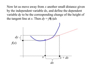
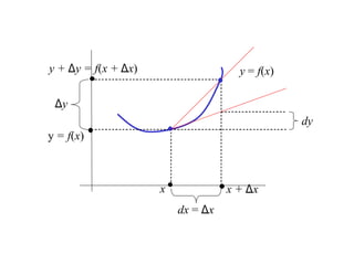
![Sometimes, instead of estimating the absolute error, we are more
interested in the relative errors
dx and dy = d [ f (x )]
y
f ( x)
x
If these are multiplied by 100 to express them as percents, we
call them the percentage errors.If we are given the maximum
percentage error of the measurement, then we want to estimate
the maximum percentage error in the computed result.](https://image.slidesharecdn.com/locallinearapproximation-140129105522-phpapp02/85/Local-linear-approximation-22-320.jpg)

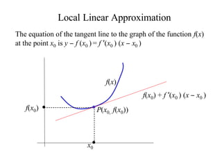
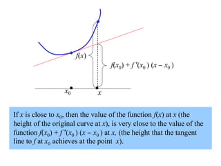
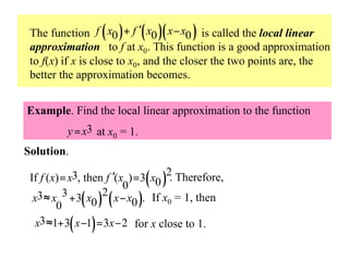
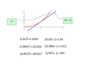
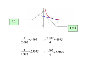
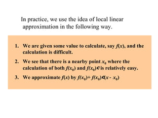
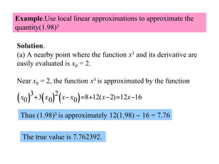
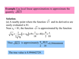
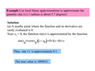
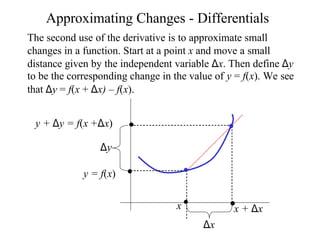
The document discusses local linear approximations, which provide a linear function that closely approximates a given non-linear function near a specific point. It defines the local linear approximation at a point x0 as f(x0) + f'(x0)(x - x0). Graphs and examples are provided to illustrate how the local linear approximation can be used to estimate function values close to x0. The concept of differentials is also introduced to estimate small changes in a function using its derivative. Examples demonstrate using differentials to approximate changes and estimate errors in computations involving measured values.