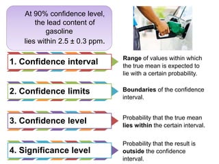
![1. Calculate the molar concentration of 8.45 (0.473%) mL
0.2517 (1.82%) g/mL ammonia solution that was
diluted to 0.5000 (0.0002) L.
(Ans. 0.250 (0.005) M)
2. Consider the function pH= –log[H+], where [H+] is the
molarity of H+. For pH = 5.21 0.03, find [H+] and its
uncertainty.
(Ans. 6.2 (0.4) x 10-6)
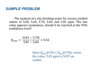
SAMPLE PROBLEM](https://image.slidesharecdn.com/statisticalanalysisinanalyticalchemistry-180125105810/85/Statistical-analysis-in-analytical-chemistry-12-320.jpg)


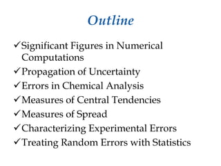
This document provides an outline and overview of key concepts related to experimental errors and statistics. It discusses significant figures in calculations, propagation of uncertainty, measures of central tendency and spread, characterizing experimental errors, and treating random errors with statistics. Specific topics covered include calculating uncertainties, confidence intervals, normal distributions, and distinguishing between random and systematic errors. The document uses examples and sample problems to illustrate key points about analyzing and interpreting experimental data.