Downloaded 10 times

![WORLD ECONOMIC OUTLOOK: War Sets Back the Global Recovery
28 International Monetary Fund | April 2022
involve a disproportionate share of contact-intensive,
physically strenuous, less flexible, and low-paying
jobs, such as in accommodation and food services and
retail trade.
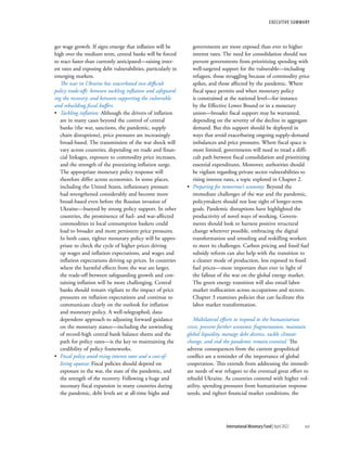
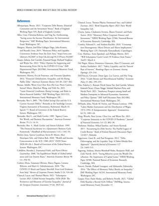
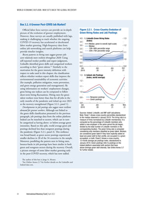
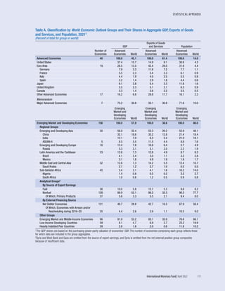
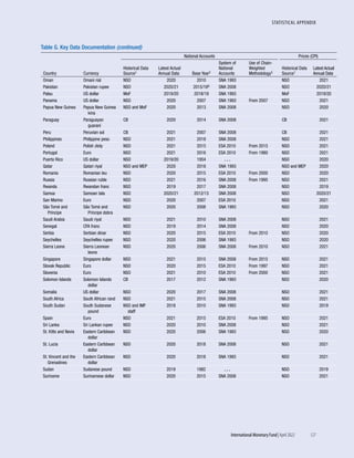
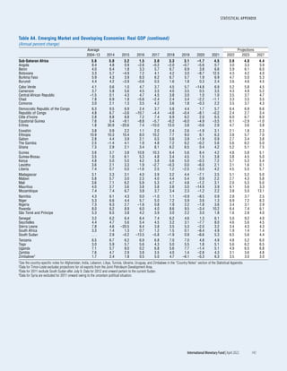
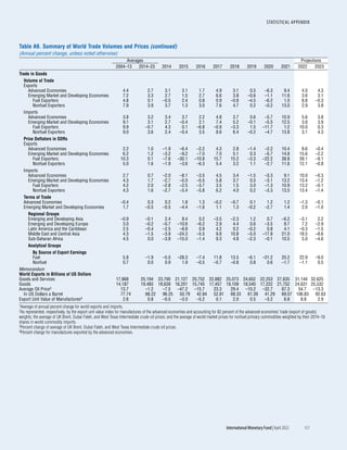
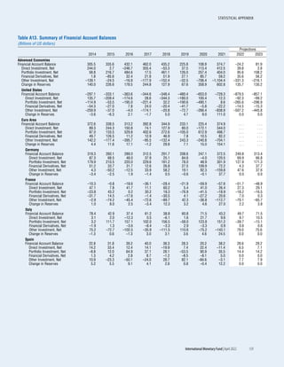
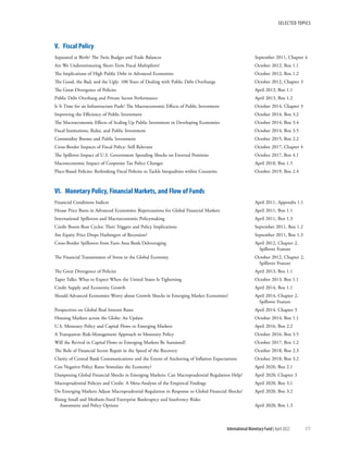
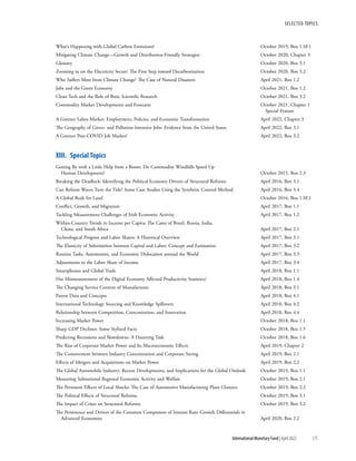
Rising labor market tightness has spurred faster
nominal wage growth, particularly for low-paying
jobs.3 Since the start of the pandemic, the increase
in tightness alone is estimated to have directly
increased overall nominal UK and US wage inflation
3In the United Kingdom and the United States, nominal
wages are already growing faster than before the pandemic,
although these gains have been largely or more than fully eroded
by price inflation. (See Duval and others [2022] for more
discussion.)
by
approximately 1.5 percentage points. In low-pay
industries, this impact has been much greater, reflect-
ing both above-average increases in labor market tight-
ness and a stronger historical link between tightness
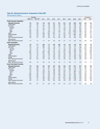
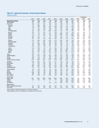
and wage growth in these industries (Figure 1.1.3). So
far, overall implications of increased tightness for wage
inflation have been muted, partly because low-wage
workers account for a relatively small share of firms’
total labor costs. To the extent that tightness remains
concentrated primarily in these jobs, the pass-through
from wage growth in low-pay occupations to
economy-wide price inflation is likely to remain
limited. However, with price inflation largely or (more
than) fully outpacing wage increases so far, and given
persistent labor markets, overall nominal wage growth
is likely to remain solid. Workers’ demands for a pay
raise to compensate for fast-rising prices, along with an
increase in their inflation expectations, could intensify
inflation pressure, more so than tight labor markets.
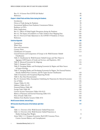
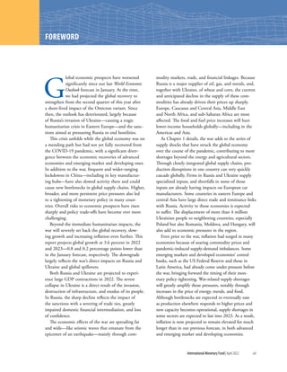
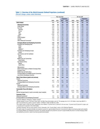
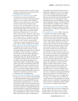
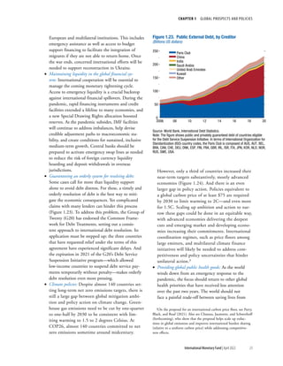
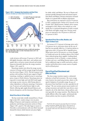
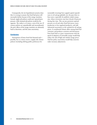
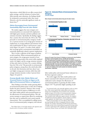
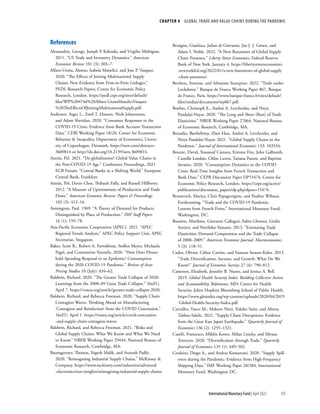
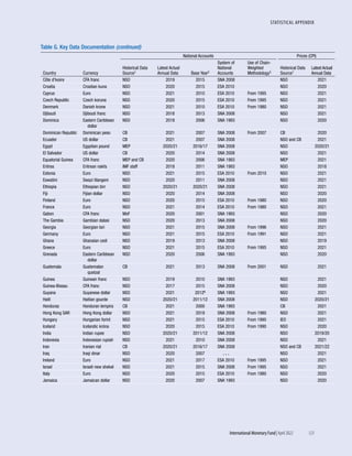
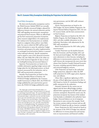
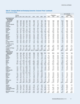
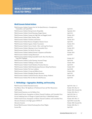
United States United Kingdom
United States trend United Kingdom trend
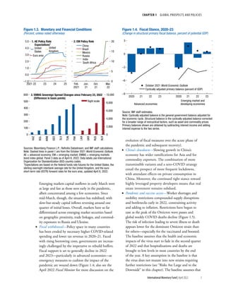
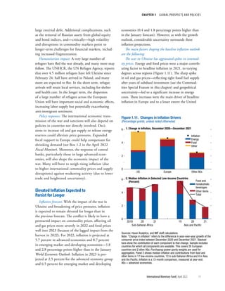
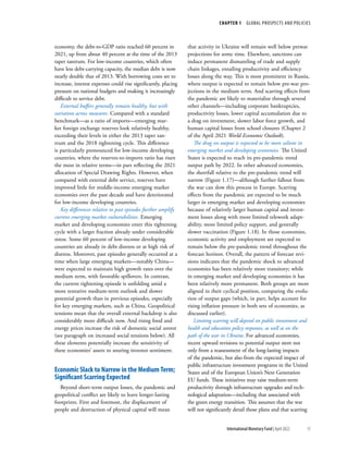
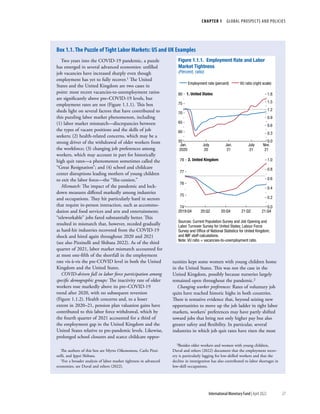
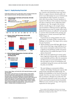
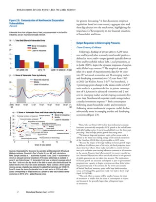
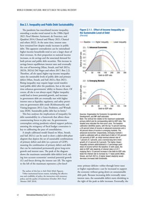
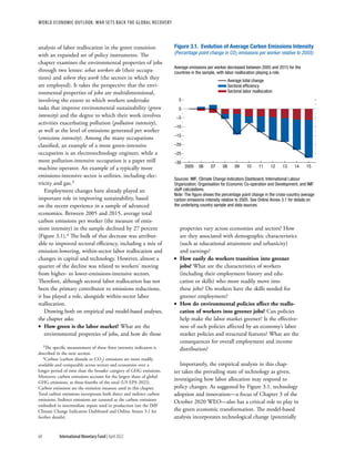
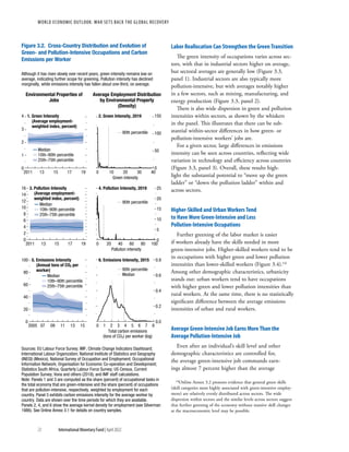
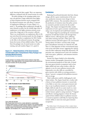
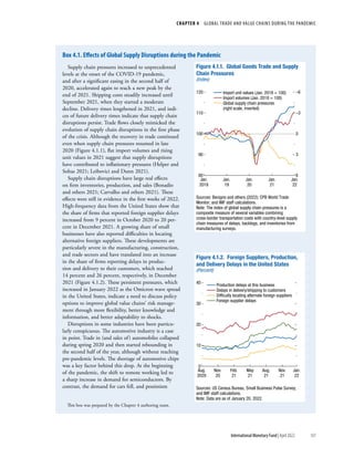
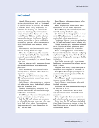
Figure 1.1.2. Inactivity Rates
(Percent)
48
50
52
54
56
58
2019:Q1 20:Q1 21:Q1 21:Q4
1. Older Workers
15
20
25
30
35
2019:Q1 20:Q1 21:Q1 21:Q4
2. Mothers with Young Children
Sources: Current Population Survey and Job Opening and
Labor Turnover Survey for United States; Labour Force
Survey and Office of National Statistics for United Kingdom;
and IMF staff calculations.
Note: Older workers are aged 55–74; young children are
aged 5 or younger. Linear trends are estimated over
2015–19.
Sources: Current Population Survey; Job Opening and Labor
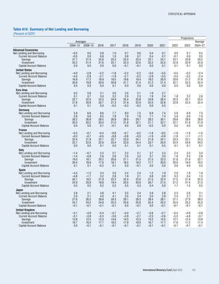
Turnover Survey; and IMF staff calculations.
Note: Wage growth is year-over-year quarterly nominal
hourly wage inflation. Tightness (measured as the
vacancy-to-unemployment ratio) is lagged one quarter
between 2003:Q1 and 2020:Q1. Each dot represents the
mean of the x-axis and y-axis variables for each of the 40
equal-sized bins of the x-axis variable. Low-pay industries
are accommodation and food services, retail trade, and arts
and entertainment.
Wage
growth
(percent)
Low-pay industries
Other industries
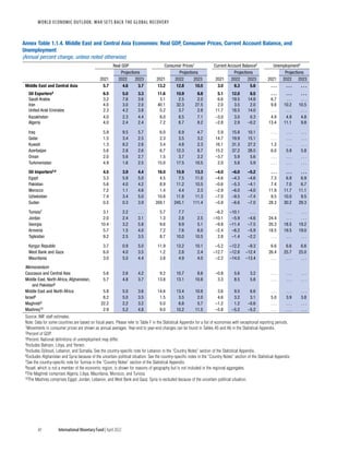
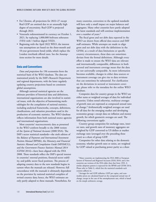
Figure 1.1.3. United States Wage Growth and
Tightness across Sectors
(Percent, ratio)
–3
–2
–1
0
1
2
3
4
5
6
0.0 0.5 1.0 1.5 2.0 2.5 3.0
Labor market tightness (ratio)
Box 1.1 (continued)](https://image.slidesharecdn.com/worldeconomicoutlook2022-imf-220627053618-c9aeb3e7/85/WORLD-ECONOMIC-OUTLOOK-2022-47-320.jpg)

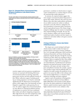
![International Monetary Fund | April 2022 45
During the pandemic, and in particular its most acute
phase, government policies helped maintain private
access to credit, staving off a deeper recession in 2020.
This chapter examines whether the resulting increase
in leverage may affect the pace of the recovery. On
average, the drag on future GDP growth is estimated
at 0.9 percent over three years for advanced econo-
mies and at 1.3 percent for emerging markets. How-
ever, analyses based on micro-level data show that the
recovery is likely to be slower in countries where (1)
leverage is concentrated among vulnerable firms and
low-income households, (2) insolvency procedures are
inefficient, (3) public and private deleveraging coincide,
and (4) monetary policy must be tightened rapidly. As
countries prepare to normalize monetary policy, assess-
ing how leverage is distributed is key to forecasting the
pace of the recovery and calibrating the unwinding of
pandemic-time support. In some advanced economies
where the recovery is well underway and private balance
sheets are in good shape, fiscal support can be reduced
faster, facilitating the work of central banks. Elsewhere,
targeted fiscal support—within the limit of a credi-
ble medium-term fiscal framework—could be relied
on to minimize the risk of disruptions and scarring.
Introduction
Accommodative policies during the acute phase of
the COVID-19 crisis mitigated its overall economic
cost by providing ample and cheap liquidity to affected
households and firms. But these policies also led to
rapid debt buildup, extending a steady rise in overall
leverage encouraged by supportive financial condi-
tions since the global financial crisis of 2008. The
surge in global private debt in 2020—13 percent of
GDP—was widespread, faster than during the global
financial crisis and almost as large as the rise in public
debt (Figure 2.1, panel 1). Nonfinancial corporations,
which entered the pandemic with already-elevated debt
The authors of this chapter are Silvia Albrizio, Sonali Das,
Christoffer Koch, Jean-Marc Natal (lead), and Philippe Wingender,
with support from Evgenia Pugacheva and Yarou Xu. They thank
Ludwig Straub for very helpful comments on an earlier draft.
(Global Financial Stability Report [GFSR], April and
October 2021), saw larger increase in debt ratios than
households. This was especially the case in advanced
economies thanks to extensive credit guarantees, con-
cessional lending programs, and moratoriums (Fig-
ure 2.1, panel 2).
Will these developments have a bearing on the
nature of the recovery that lies ahead? After all,
one person’s debt is another person’s asset, so why
should it matter?
Answers to these questions require delving deep
into why private debt matters. First, it matters
because debtors and creditors are not alike.1 Bor-
rowers are typically constrained financially, with the
severity of the constraint depending on the financial
resources at their command. High-net-worth, liquid
households and firms can sustain large variations in
indebtedness with minor consequences for spending;
higher debt often finances the accumulation of assets
that can later be drawn down to finance consumption
or investment. Low-net-worth, illiquid households
and firms, on the other hand, are more constrained.
They are also more sensitive to leverage cycles and
more reactive to changes in fiscal and monetary poli-
cies. Such distinction is particularly relevant if rising
interest rates lead to conditions and financial instabil-
ity (April 2022 GFSR and Chapter 1).
Second, periods of rapidly increasing debt may
become unsustainable and lead to periods of deleverag-
ing accompanied by subpar growth. In a nutshell, loose
financial conditions encourage debt buildup, which
boosts spending, growth, and asset prices and further
incentivizes credit as collateral values increase. This
eventually unwinds when returns disappoint or are too
poor to justify further debt-financed investment, lend-
ers become wary of rolling over credit and extending
new loans, or financial conditions tighten and rising
debt-service costs crowd out other spending.
1Tobin (1980) argues that “the population is not distributed
between debtors and creditors randomly. Debtors have borrowed for
good reasons, most of which indicate a high marginal propensity to
spend from wealth or from current income or from any other liquid
resources they can command.”
PRIVATE SECTOR DEBT AND THE GLOBAL RECOVERY
2
CHAPTER](https://image.slidesharecdn.com/worldeconomicoutlook2022-imf-220627053618-c9aeb3e7/85/WORLD-ECONOMIC-OUTLOOK-2022-64-320.jpg)
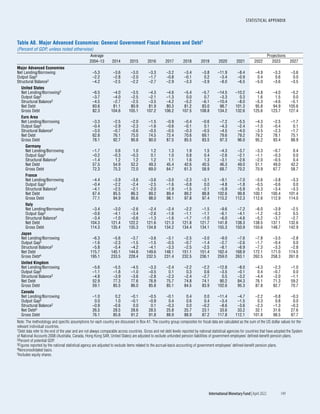
![CHAPTER 2 PRIVATE SECTOR DEBT AND THE GLOBAL RECOVERY
47
International Monetary Fund | April 2022
Leverage cycles, heterogeneity, and future growth:
Current levels of private leverage are expected to
exert some drag on future GDP growth. Estimates
based on cross-country aggregate data point to a
cumulative 0.9 percent slowdown over three years
for advanced economies and a cumulative 1.3 per-
cent slowdown for emerging markets. However, the
post-pandemic drag on growth could be much larger
in countries where (1) indebtedness is more concen-
trated among financially constrained households and
vulnerable firms, (2) the insolvency regime is inef-
ficient, (3) fiscal space is limited, and (4) monetary
policy needs to be tightened rapidly. For example,
a surprise tightening of 100 basis points is esti-
mated to slow investment among highly leveraged
firms by a cumulative 6½ percentage points over
two years, 4 percentage points more than among
those with little leverage. The effect could be larger
if higher interest rates lead to financial instability
(April 2021 GFSR).
Implications for policy: Stronger emphasis on distri-
butional considerations for macroeconomic forecasting
and policymaking is needed. For example, where the
recovery is well underway and private balance sheets
are in good shape—mainly in advanced economies that
benefited from generous government support during
the pandemic—fiscal support can be reduced faster,
facilitating the work of central banks. Elsewhere, the
recovery may be weaker, and targeted fiscal support
could help lessen the risks of disruptions and scarring
within credible medium-term fiscal frameworks (April
2022 Fiscal Monitor). Where targeting is difficult and
fiscal space limited, countries may need to consider
revenue-enhancing measures to fund various priorities.
Increasing tax compliance and other reforms to mod-
ernize business taxation are possible avenues; the latter
could include temporary increases in corporate income
tax designed to capture pandemic-related excess profits
(IMF 2021a).
This chapter builds on earlier IMF work (April
2021 GFSR; April 2012 and April 2020 World
Economic Outlook [WEO]; October 2020 Regional
Economic Outlook: Europe; October 2020 Regional Eco-
nomic Outlook: Western Hemisphere) and draws on two
strands of literature that emphasize the importance
of heterogeneity (Jappelli and Pistaferri 2014; Cloyne
and others 2018; Kaplan, Moll, and Violante 2018;
Ottonello and Winberry 2020) and leverage (Bernanke,
Gertler, and Gilchrist 1999; Iacoviello 2005;
Eggertsson and Krugman 2012; Jordà, Schularick, and
Taylor 2011; Dell’Ariccia and others 2016; Mian, Sufi,
and Verner 2017; Drehman, Juselius, and Korinek
2017) in the transmission and amplification of eco-
nomic shocks and policy.
The chapter starts by highlighting recent develop-
ments in households’ and nonfinancial corporations’
balance sheets, focusing on the distribution of debt.
Cross-country panel regressions estimate the macroeco-
nomic impact of leverage buildup on future growth.
Micro-level data on households and firms then help
unpack the role of heterogeneity and the importance
of countercyclical and structural policy.
Private Sector Leverage during the Pandemic
This section sheds light on the historical devel-
opment of household and corporate balance sheets,
focusing on the COVID-19 recession and buildup of
leverage among heterogeneous households and firms.
Household Balance Sheets
A Global Cycle in Assets and Liabilities
Household balance sheets have expanded almost
continuously in recent decades, with net wealth
increasing globally from an average 225 percent of
GDP in 1995 to more than 360 percent of GDP in
2020, in purchasing-power-parity-weighted terms.
Nevertheless, household debt has passed through two
distinct phases over the past two decades. Among
advanced economies, household leverage increased
steadily in the years before the global financial crisis.
Since debt was used primarily to finance housing
investment, this resulted in assets growing in tandem
with liabilities (Figure 2.2). In the decade after the
global financial crisis, households gradually reduced
debt relative to income, and housing assets also fell
relative to income, with the reductions driven by
lower valuations and slower investment. House-
hold debt jumped in 2020 because of increased
borrowing and lower income as a result of the
pandemic-induced recession. This rise in debt was
accompanied by a large increase in financial assets.
Looking ahead, net wealth could contract again as
governments’ cash transfers to households stop, and
tighter financial conditions may increase debt-service
costs and lead to declines in asset prices (see the April
2022 GFSR).](https://image.slidesharecdn.com/worldeconomicoutlook2022-imf-220627053618-c9aeb3e7/85/WORLD-ECONOMIC-OUTLOOK-2022-66-320.jpg)
![CHAPTER 2 PRIVATE SECTOR DEBT AND THE GLOBAL RECOVERY
49
International Monetary Fund | April 2022
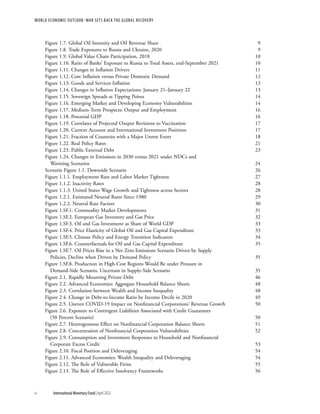
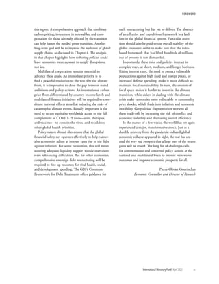
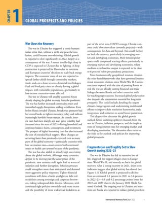
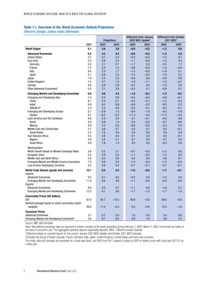
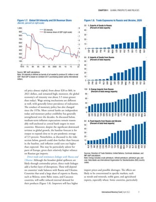
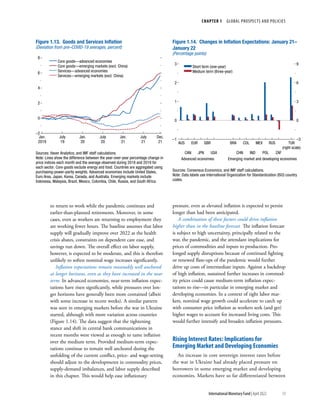
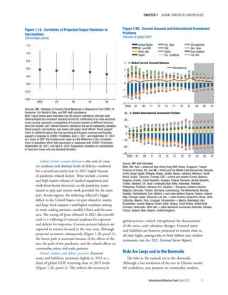
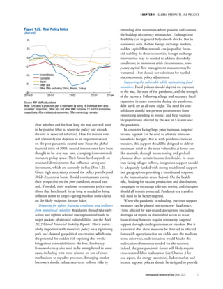
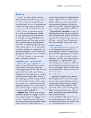
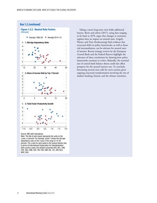
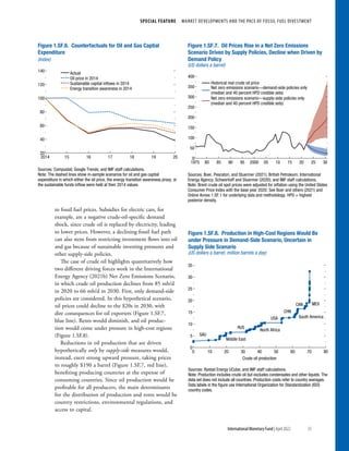
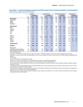
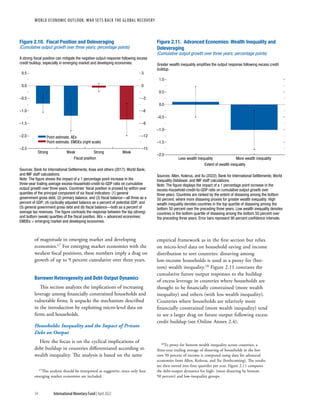
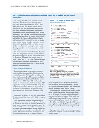
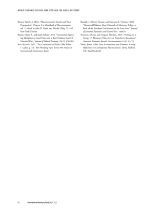
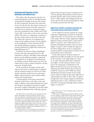
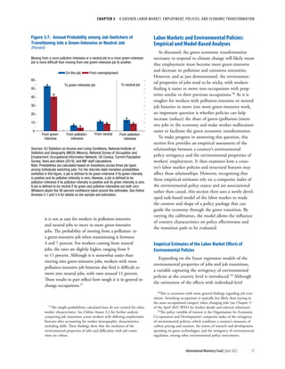
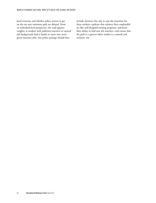
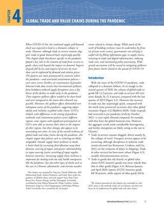
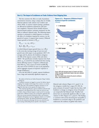
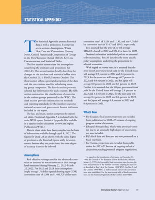
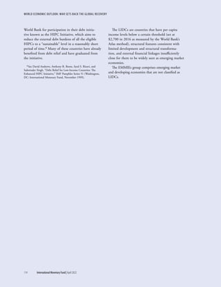
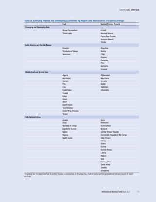
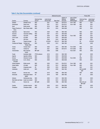
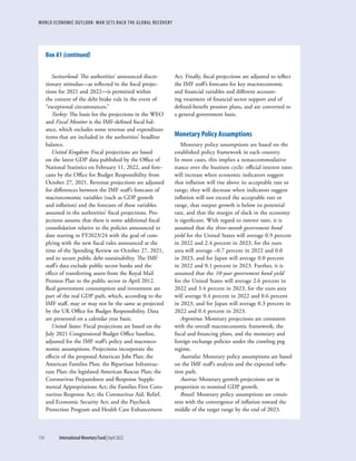
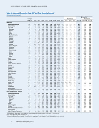
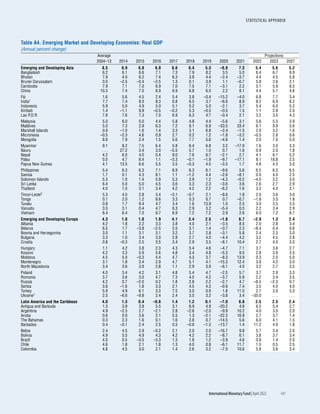
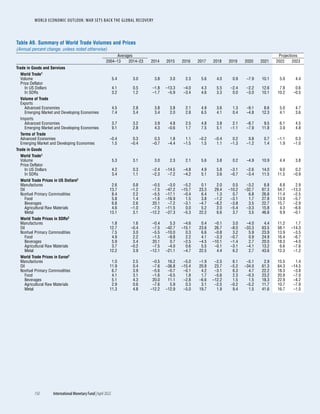
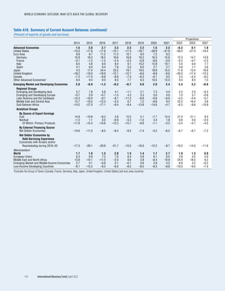
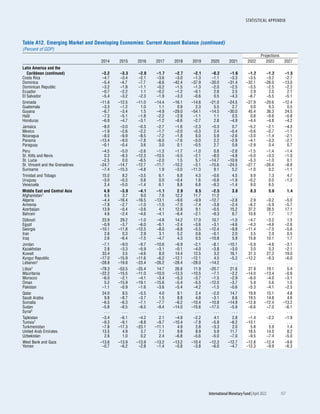
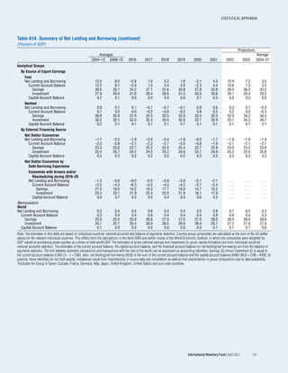
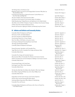
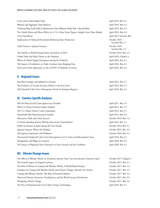
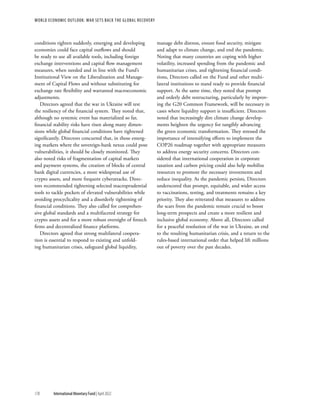
Despite smaller aggregate increases in debt ratios
in Germany, the United Kingdom, and Hungary and
even outright decline in the United States, low-income
households saw comparatively larger increases in debt.
The buildup exceeded 10 percent of income in the
United States for households with incomes below
$15,000. In the United Kingdom, debt increased by
about 7.5 percent of income for households in the
lowest tercile. In contrast, France and Italy were able to
support low- and middle-income households’ balance
sheets, as seen from the decline in debt ratios in both
countries for the bottom 50 percent of incomes.
This exercise is possible only for the small number
of countries that conducted household wealth surveys
in the past. As attention to inequality and distribu-
tional issues increases, the expansion of data collection
on household balance sheets will allow a better under-
standing of the impact of shocks and policies.
Firms’Balance Sheets
Concentrated Vulnerabilities in the Nonfinancial
Corporate Sector
Abundant liquidity support through loans, credit
guarantees, and moratoriums on debt repayment con-
tributed to debt buildup and was pivotal in preventing
widespread corporate failures and related employment
and output losses, especially among small and medium
enterprises. The analysis here takes stock of balance
sheet developments since the pandemic began, with a
focus on the distribution of leverage and vulnerabilities
across firms, sectors, and countries.
Figure 2.5 uses publicly listed firms’ quarterly balance
sheets4 to present revenue growth by sector across 71
advanced and emerging market economies in 2020 and
compares this with 2009, at the height of the global
financial crisis. A clear sectoral contrast emerges. Because
of lockdowns or materials shortages, the largest losses
are concentrated in a few sectors, such as consumer
services, transportation, automobiles, and components.
In contrast, at the other end of the distribution, some
sectors gained from the structural pivot imposed by the
pandemic (semiconductors, software and information
technology [IT] services, pharmaceuticals and biotech-
nology, and health care equipment and services). This
is different from what took place during the global
financial crisis, when the shock hit almost all the sectors
considered. Moreover, a substantial part of the increase
in leverage during the pandemic was covered by gov-
ernment guarantees.5 Therefore, the risk of an adverse
feedback loop in which corporate distress puts stress on
the financial system—and eventually the public purse—
appears smaller, at least in countries where the govern-
ment can absorb the shock (Chapter 2 in the April 2022
GFSR analyzes risks associated with the sovereign-bank
nexus in emerging markets). Figure 2.6 suggests that the
biggest commitments were made in advanced econ-
omies, where fiscal space is the largest (see Box 2.1).
However, it is worth noting that regulatory forbearance
may have masked the real extent of losses.
4Standard & Poor’s Capital IQ data are used in the whole subsection
for their timeliness. But since they only comprise firms listed on stock
exchanges, they cover only 7 percent of total employment. This suggests
the reported share of firms in the worst-hit sectors should be considered
a lower bound given that small and medium enterprises, which account
for large labor and value-added shares in some of the economies, are
not included in the sample. See Online Annex 2.1 for details.
5The share of those guarantees in total credit is highly variable,
ranging from about 20 percent of all new credit in Germany to
100 percent (up to a certain limit) in Japan.
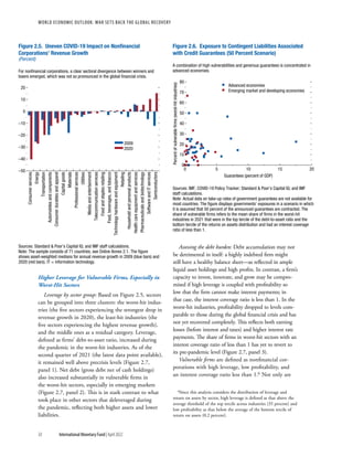
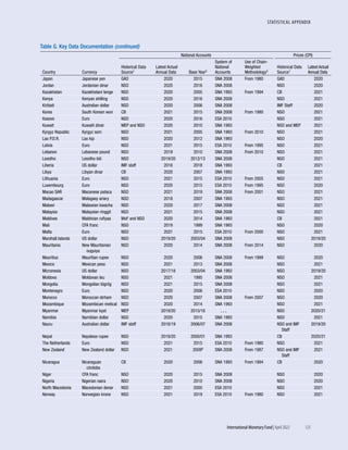
USA FRA ITA GBR DEU
CHN HUN ZAF
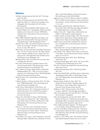
Figure 2.4. Change in Debt-to-Income Ratio by Income Decile
in 2020
(Percent of income)
Household indebtedness varied across countries and household income groups.
1. Advanced Economies
–20
–10
0
10
20
1 3 5 7 9
2 4 6 8 10
2. Emerging Market Economies
–20
–10
0
10
20
1 3 5 7 9
2 4 6 8 10
Source: IMF staff calculations.
Note: Income deciles on x-axes, except for the United States where households
are grouped by fixed income bands. See Online Annex 2.1. CHN = China;
DEU = Germany; FRA = France; GBR = United Kingdom; HUN = Hungary;
ITA = Italy; USA = United States; ZAF = South Africa.](https://image.slidesharecdn.com/worldeconomicoutlook2022-imf-220627053618-c9aeb3e7/85/WORLD-ECONOMIC-OUTLOOK-2022-68-320.jpg)
![WORLD ECONOMIC OUTLOOK: War Sets Back the Global Recovery
86 International Monetary Fund | April 2022
Hobijn, Bart, and Ayşegül Şahin. 2009. “Job-Finding and
Separation Rates in the OECD.” Economics Letters 104
(2009): 107–11.
Intergovernmental Panel on Climate Change (IPCC). 2015.
Climate Change 2014: Mitigation of Climate Change; Working
Group III Contribution to the IPCC Fifth Assessment Report.
New York: Cambridge University Press.
Intergovernmental Panel on Climate Change (IPCC). 2018.
Global Warming of 1.5°C: An IPCC Special Report on the
Impacts of Global Warming of 1.5°C above Pre-industrial Levels
and Related Global Greenhouse Gas Emission Pathways, in
the Context of Strengthening the Global Response to the Threat
of Climate Change, Sustainable Development, and Efforts to
Eradicate Poverty, edited by V. Masson-Delmotte, P. Zhai,
H.-O. Pörtner, D. Roberts, J. Skea, P. R. Shukla, A. Pirani,
and others. Geneva.
International Energy Agency (IEA). 2021. “The Cost of Capital
in Clean Energy Transitions.” https://
www
.iea
.org/
articles/
the
-cost
-of
-capital
-in
-clean
-energy
-transitions. Paris.
International Monetary Fund (IMF). 2022. France: Selected
Issues. IMF Staff Country Report 22/19. Washington, DC.
Karabarbounis, Loukas, and Brent Neiman. 2014. “The Global
Decline of the Labor Share.” Quarterly Journal of Economics
129 (1): 61–103.
Levy Yeyati, Eduardo, Martín Montané, and Luca Sartorio.
2019. “What Works for Active Labor Market Policies?”
Center for International Development at Harvard Faculty
Working Paper 358, Harvard University, Cambridge, MA.
Martin, John P. 1996. “Measures of Replacement Rates for the
Purpose of International Comparisons: A Note.” OECD
Economic Studies 26: 99–115.
Observatoire National des Emplois et Métiers de l’Economie
Verte (ONEMEV). 2021. “Métiers Verts et Verdissants: Près
de 4 Millions de Professionnels en 2018” [Green and Greening
Professions: Nearly 4 Million Professionals in 2018]. https://
www
.statistiques
.developpement
-durable
.gouv
.fr/
metiers
-verts
-et
-verdissants
-pres
-de
-4
-millions
-de
-professionnels-en-2018.
Organisation for Economic Co-operation and Development
(OECD). 1994. The OECD Jobs Study: Facts, Analysis,
Strategy. Paris.
Organisation for Economic Co-operation and Development
(OECD) and European Centre for the Development of Voca-
tional Training (Cedefop). 2014. Greener Skills and Jobs. Paris.
O*NET Center. 2010. “Green Task Development Project.”
https://
www
.onetcenter
.org/
reports/
GreenTask
.html. Accessed
May 17, 2021.
O*NET Center. 2021. “Green Occupations.” Version 22.0.
https://
www
.onetcenter
.org/
dictionary/
22
.0/
excel/
green
_occupations.html.
Silverman, Bernard W. 1986. Density Estimation for Statistics and
Data Analysis. London: Chapman and Hall.
United States Environmental Protection Agency (US EPA).
2022. “Global Greenhouse Gas Emissions Data.” https://
www
.epa
.gov/
ghgemissions/
global
-greenhouse
-gas
-emissions
-data.
Washington, DC.
van der Velden, Rolf, and Ineke Bijlsma. 2016. “College Wage
Premiums and Skills: A Cross-Country Analysis.” Oxford
Review of Economic Policy 32 (4): 497–513.
Vona, Francesco, Giovanni Marin, and Davide Consoli. 2019.
“Measures, Drivers, and Effects of Green Employment: Evi-
dence from US Local Labor Markets, 2006–2014.” Journal of
Economic Geography 19 (5): 1021–48.
Vona, Francesco, Giovanni Marin, Davide Consoli, and David
Popp. 2018. “Environmental Regulation and Green Skills: An
Empirical Exploration.” Journal of the Association of Environ-
mental and Resource Economists 5 (4): 713–53.](https://image.slidesharecdn.com/worldeconomicoutlook2022-imf-220627053618-c9aeb3e7/85/WORLD-ECONOMIC-OUTLOOK-2022-105-320.jpg)

![STATISTICAL APPENDIX
International Monetary Fund|April 2022 113
In 2019 Zimbabwe authorities introduced the Real
Time Gross Settlement dollar, later renamed the Zim-
babwe dollar, and are in the process of redenominating
their national accounts statistics. Current data are sub-
ject to revision. The Zimbabwe dollar previously ceased
circulating in 2009, and during 2009–19, Zimbabwe
operated under a multicurrency regime with the US
dollar as the unit of account.
Classification of Countries
Summary of the Country Classification
The country classification in the WEO divides the
world into two major groups: advanced economies
and emerging market and developing economies.6 This
classification is not based on strict criteria, economic
or otherwise, and it has evolved over time. The objec-
tive is to facilitate analysis by providing a reasonably
meaningful method of organizing data. Table A pro-
vides an overview of the country classification, showing
the number of countries in each group by region and
summarizing some key indicators of their relative size
(GDP valued at purchasing power parity, total exports
of goods and services, and population).
Some countries remain outside the country classifica-
tion and therefore are not included in the analysis. Cuba
and the Democratic People’s Republic of Korea are
examples of countries that are not IMF members, and
the IMF therefore does not monitor their economies.
General Features and Composition of Groups in
the World Economic Outlook Classification
Advanced Economies
Table B lists the 40 advanced economies. The seven
largest in terms of GDP based on market exchange
rates—the United States, Japan, Germany, France,
Italy, the United Kingdom, and Canada—constitute
the subgroup of major advanced economies, often
referred to as the Group of Seven. The members of
the euro area are also distinguished as a subgroup.
Composite data shown in the tables for the euro area
cover the current members for all years, even though
the membership has increased over time.
6 As used here, the terms “country” and “economy” do not always
refer to a territorial entity that is a state as understood by interna-
tional law and practice. Some territorial entities included here are
not states, although their statistical data are maintained on a separate
and independent basis.
Table C lists the member countries of the European
Union, not all of which are classified as advanced
economies in the WEO.
Emerging Market and Developing Economies
The group of emerging market and developing
economies (156) includes all those that are not classi-
fied as advanced economies.
The regional breakdowns of emerging market and
developing economies are emerging and developing
Asia; emerging and developing Europe (sometimes
also referred to as “central and eastern Europe”); Latin
America and the Caribbean; Middle East and Central
Asia (which comprises the regional subgroups Caucasus
and Central Asia; and Middle East, North Africa,
Afghanistan, and Pakistan); and sub-Saharan Africa.
Emerging market and developing economies are also
classified according to analytical criteria that reflect
the composition of export earnings and a distinc-
tion between net creditor and net debtor economies.
Tables D and E show the detailed composition of
emerging market and developing economies in the
regional and analytical groups.
The analytical criterion source of export earnings
distinguishes between the categories fuel (Standard
International Trade Classification [SITC] 3) and
nonfuel and then focuses on nonfuel primary products
(SITCs 0, 1, 2, 4, and 68). Economies are categorized
into one of these groups if their main source of export
earnings exceeded 50 percent of total exports on aver-
age between 2016 and 2020.
The financial and income criteria focus on net credi-
tor economies, net debtor economies, heavily indebted
poor countries (HIPCs), low-income developing countries
(LIDCs), and emerging market and middle-income
economies (EMMIEs). Economies are categorized as net
debtors when their latest net international investment
position, where available, was less than zero or their
current account balance accumulations from 1972
(or earliest available data) to 2020 were negative. Net
debtor economies are further differentiated on the basis
of experience with debt servicing.7
The HIPC group comprises the countries that
are or have been considered by the IMF and the
7 During 2016–20, 35 economies incurred external payments
arrears or entered into official or commercial bank debt-rescheduling
agreements. This group is referred to as economies with arrears and/or
rescheduling during 2016–20.](https://image.slidesharecdn.com/worldeconomicoutlook2022-imf-220627053618-c9aeb3e7/85/WORLD-ECONOMIC-OUTLOOK-2022-132-320.jpg)

The document is the April 2022 edition of the World Economic Outlook report published by the International Monetary Fund. It finds that the war in Ukraine has set back the global recovery from the COVID-19 pandemic. The report forecasts slower global growth in 2022 and 2023, rising inflation pressures that are likely to persist, and increased financial vulnerabilities for emerging markets due to rising interest rates. It calls for policies to sustain the recovery through investment in green energy transitions and strengthening social safety nets, while improving fiscal positions in the medium term.


