OptimJ is an extension of Java for writing optimization models, supporting bulk data processing and algebraic modeling similar to other languages like AIMMS and GAMS. It operates directly on Java objects and includes integration with various optimization engines such as LP_Solve and Gurobi, as well as offering a familiar programming environment through the Eclipse IDE. The manual provides a comprehensive overview of OptimJ features, installation guidance, and coding constructs for creating optimization models.


![3 Language constructs for modeling
3.1 The basics : optimization concepts in Java
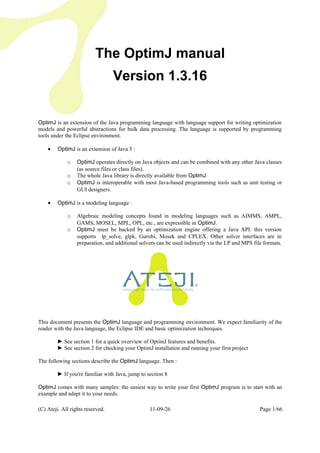
An OptimJ program combines Java code and optimization code. Here is a basic example:
(C) Ateji. All rights reserved. 11-09-26 Page 8/66
package examples;
// a simple model for the map-coloring problem
public model SimpleColoring solver lpsolve
{
// maximum number of colors
int nbColors = 4;
// decision variables hold the color of each country
var int belgium in 1 .. nbColors;
var int denmark in 1 .. nbColors;
var int germany in 1 .. nbColors;
// neighbouring countries must have a different color
constraints {
belgium != germany;
germany != denmark;
}
// a main entry point to test our model
public static void main(String[] args)
{
// instanciate the model
SimpleColoring m = new SimpleColoring();
// solve it
m.extract();
m.solve();
// print solutions
System.out.println("Belgium: " + m.value(m.belgium));
System.out.println("Denmark: " + m.value(m.denmark));
System.out.println("Germany: " + m.value(m.germany));
}
}
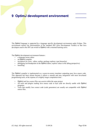
First OptimJ program : a simple model for the map coloring problem.](https://image.slidesharecdn.com/optimjmanualv1-170223214034/85/The-OptimJ-Manual-8-320.jpg)
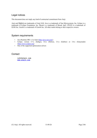
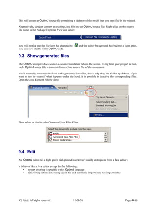
![3.3 Solver context
Some concepts such as instanciation of a decision variable or creation of a constraint make sense only in
relation with a given solver. In order to handle this restriction, OptimJ introduces the notion of a solver
context.
A solver context is introduced by the model declaration with the keyword solver :
The scope of the solver context is the fields of the model, the constraints blocks and the objective clause.
The solver context cannot be redefined – this is why a model cannot extend a model.
The solver context puts restrictions on the types allowed for decision variables, on the operations allowed
for writing constraints, and on the structure of constraints (linear, quadratic, etc.).
The solver context specifies the methods that can be invocated on decision variables. It also defines a
“solver object”, accessible through the method solver(), and the methods that it provides (see section 4).
This is OptimJ's way of bringing into the language all the solver specific APIs.
(C) Ateji. All rights reserved. 11-09-26 Page 10/66
model SimpleColoring solver lpsolve
{
...
}
Introducing a solver context
// this example shows the parts impacted by the choice of a solver
import lpsolve.LpSolve;
model Coloring solver lpsolve
{
var double x; // OK, lpsolve handles double variables
constraints {
2*x <= 3; // OK, lpsolve handles linear constraints
}
public static void main(String[] args)
{
// here we instanciate the model : its type is 'Coloring'
Coloring coloring = new Coloring();
// extracting the model also instanciates the solver
coloring.extract();
// here we get the instance of the solver :
// its type depends on the choosen solver
LpSolve mySolver = coloring.solver();
}
}
Introducing a solver context](https://image.slidesharecdn.com/optimjmanualv1-170223214034/85/The-OptimJ-Manual-10-320.jpg)
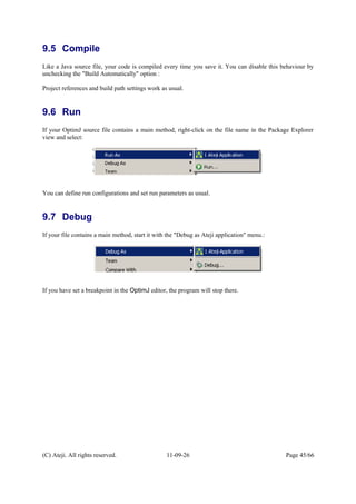
![Var types are the types of decision variables. They are written var T, where T is any Java type.
var is a type functional taking a type argument – it is not a declaration modifier. var is left-associative,
meaning that var int[] is to be read as an array of var int, not as a var type ranging over int[].
In the example above, OptimJ will complain that some variables need a domain : read on.
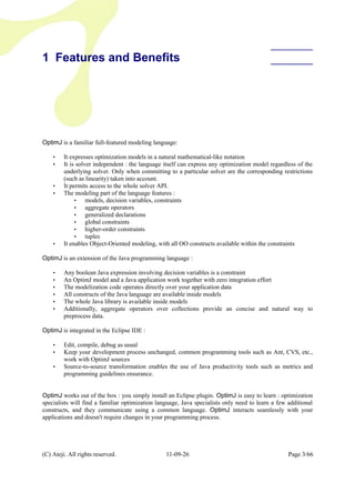
3.4.2 Declaring decision variables
Decision variables or arrays thereof must be declared as fields of a model (they cannot be declared as e.g.
local variables of a method).
A decision variable is always initialized. If you do not provide an initialization, OptimJ will do it for you
if the variable is numeric or boolean.
You can think of decision variables as Java objects, which can be initialized with constructors of the
appropriate type. The constructors will require you to provide a domain for each decision variable : the
domain is the set of all possible solution values. For numeric types, OptimJ provides a familiar notation
where you simply provide the bounds.
The exact set of constructors available for a given type depends on the solver context. Refer to your solver
context specification in the second part of this manual.
(C) Ateji. All rights reserved. 11-09-26 Page 12/66
String[] stringDomain = { "abc", "def" };
// Java-style initialization
var int i1 = new var int(0,10);
var double d1 = new var double(0.0, 10.0);
var String s1 = new var String(stringDomain);
// modeling-style initialization - same as above
var int i2 in 0 .. 10;
var double d2 in 0.0 .. 10.0;
var String s2 in stringDomain;
initializing decision variables
// OK: a decision variable in a field
var double d1;
// OK: an array of decision variables in a field
var double[] d2[10];
void aMethod()
{
// Wrong : a local declaration
var int d3;
}
decision variables must be fields of a model](https://image.slidesharecdn.com/optimjmanualv1-170223214034/85/The-OptimJ-Manual-12-320.jpg)
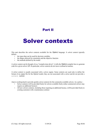
![3.4.3 Provide tight bounds
If you do not provide the domain of a numeric variable, OptimJ will provide one for you. Non-numeric
variables always require an explicit domain (there would be no way for OptimJ to guess the domain that
you intended).
Nevertheless, it is a good practice not to rely on implicit domains and always provide the tightest possible
bounds for your variables. This can considerably speed-up running times, even more so for integral
variables (whenever search is involved, the search space may grow exponentially with respect to the
domain size). OptimJ will display a warning whenever you use an implicit (unbound) domain.
3.4.4 Declaring arrays of decision variables
You can also declare arrays of decision variables. Because Java-style declarations tend to make models
unnecessarily verbose, OptimJ provides syntactic facilities known as generalized declarations.
In this exemple, we declare two arrays of ten decision variables and initialize them with their implicit
domain :
Using associative arrays (see section 6.1 for more details), you can index the array element using a string
rather than a number:
Syntax note:
Notice that the array brackets must appear twice in a generalized declaration :
• once as a type (the type of a1 is an array of var int)
(C) Ateji. All rights reserved. 11-09-26 Page 13/66
// this generalized declaration
var int[] a1[10];
// is a short-hand for the following
var int[] a2 = new var int[10];
arrays of decision variables
var int i; // in Integer.MIN_VALUE .. Integer.MAX_VALUE;
var double d; // in -Double.MAX_VALUE .. Double.MAX_VALUE;
var String s; // wrong : requires an explicit domain
implicit domains
var int[String] a3;
associative arrays of decision variables](https://image.slidesharecdn.com/optimjmanualv1-170223214034/85/The-OptimJ-Manual-13-320.jpg)
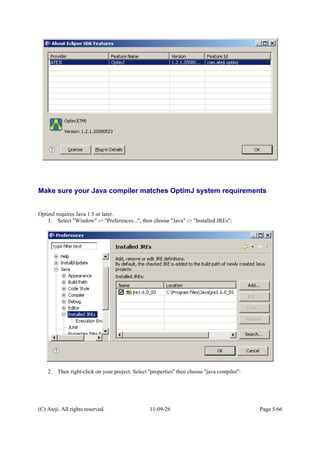
![• once as a dimensioning expression (the size of a1 is 10)
Generalized array declarations can also provide domains. In this exemple we declare an array of ten
decision variables whose domains are 0 .. 10 :
Generalized declarations can also use generators. A generator introduces a name that ranges over the array
elements, and this name can be reused in the domain expression.
In the following example, a is an array of 10 var int elements. The domain of a[0] is 0 .. 0, the domain of
a[1] is 0 .. 2, the domain of a[2] is 0 .. 4, and so on. Similarly, b is a two-dimensional array of decision
variables defined using two generators.
3.4.5 Decision variables as Java objects
Depending on the context, decision variables can also be seen as Java objects. In the following example,
the expression v.m() is in a constraints context, it refers to an invocation of the method m() in type C.
(this means intuitively that in any solution, the value of v must be such that v.m() == 0):
On the other hand, in a programming context, v is regarded as a plain Java objects having a specific
reference type var C. You can do with v everything you can do with a plain Java object.
Remember however that objects of var types can only be declared inside a solver context, which basically
means as fields of a model (they cannot be declared into a plain class).
3.5 Constraints
A constraint is any Java boolean expression involving decision variables. They have the same syntax as
ordinary Java expressions. Constraints can be written within a constraints block and only there. A
model may contain any number of constraints blocks.
The following are examples of constraints :
(C) Ateji. All rights reserved. 11-09-26 Page 14/66
var int[] a[int i : 10] in 0 .. 2*i; // i loops from 0 to 9
var int[][] b[int i : 10][int j : 10] in 0 .. i+j;
generators in generalized declarations
var int[] a[10] in 0 .. 10;
domains in generalized declarations
abstract model M {
var C v in CDomain;
constraints {
v.m() == 0;
}
}
invoking a method on a decision variable](https://image.slidesharecdn.com/optimjmanualv1-170223214034/85/The-OptimJ-Manual-14-320.jpg)
![This is the same constraint as :
This sum example is a particular case of the more general concept of comprehension, which is detailed in
section 7. The qualifier part can contain any number of generators and filters, the target part is any Java
expression.
The aggregate operators allowed for constraints depend on the solver context. Refer to your solver context
specification in the second part of this manual.
3.5.2 Collections of constraints, conditional constraints
Collections of constraints can be expressed with the forall construct, based on the same comprehension
notation :
forall constructions can be embedded and filters can be written as if clauses. This is the same as above:
Note that the if clause introducing a conditional constraint is unrelated to the if statement.
3.6 Solver-specific constraints
The OptimJ language itself is independant of any particular solver. You can however use specific
constraints (typically the so-called "global constraints") of a given solver within a constraints block by
prefixing them with the name of the solver context. Solver-specific constraints are described in each solver
(C) Ateji. All rights reserved. 11-09-26 Page 16/66
constraints {
sum{ int i : 0 .. 3 }{ gain[i] } == 0;
}
a sum constraint
constraints {
forall(Country c1 : cs, Country c2 : cs, :next(c1,c2)) {
color[c1] != color[c2];
}
}
a simple forall
constraints {
forall(Country c1 : cs) {
forall(Country c2 : cs) {
if(next(c1,c2)) {
color[c1] != color[c2];
}
}
}
}
embedded foralls and conditional constraints
constraints {
gain[0] + gain[1] + gain[2] + gain[3] == 0;
}
the same constraint fully developed](https://image.slidesharecdn.com/optimjmanualv1-170223214034/85/The-OptimJ-Manual-16-320.jpg)
![context documentation in the second part of this manual. Obviously, models using solver specific
constraints will not be portable across different solvers.
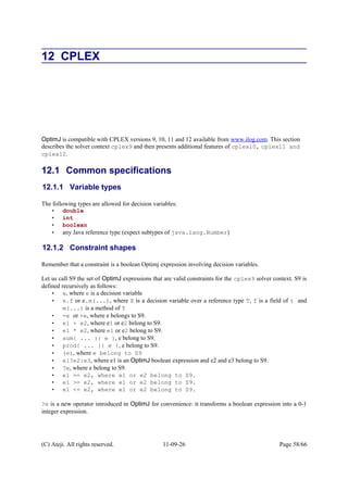
The following is an example of using a CPLEX specific SOS constraint. Note the cplex11 prefix:
3.7 Objective
The objective declaration in a model is optional. You will write one when you want to minimize or
maximize some expression (typically, you'll want to minimize a cost or maximize a profit). The expression
after the minimize or maximize keyword is any Java numeric expression involving decision variables,
exactly like a constraint.
For example, we may want to minimize the total cost of buying different foods :
3.8 Naming constraints and objective
Constraints and objective can be named. This is useful for getting information about the quality of your
solution, such as dual values. Constraint names have the type constraints. You first declare the names,
then associate them to your constraints or objective as follows :
(C) Ateji. All rights reserved. 11-09-26 Page 17/66
minimize sum{int j : nbFoods} { cost[j] * Buy[j] };
E17: objective function
model M solver cplex11
{
var int [] sosVars [10] in -5 .. 5;
double [] weights = new double [10];
constraints {
cplex11.SOS1(sosVars, weights);
}
}
example of a solver-specific constraint
// declare the names
constraints[] upperBound[nbFoods];
constraints {
forall(int j : nbFoods) {
// the j-th constraint is named upperBound[j]
upperBound[j]: Buy[j] <= max[j];
}
}
naming constraints](https://image.slidesharecdn.com/optimjmanualv1-170223214034/85/The-OptimJ-Manual-17-320.jpg)
![3.9 The model life cycle
The following is a typical example of a model life cycle :
This example demonstrates the three phases of a model life cycle:
Instantiation
This is the same as instantiating a Java class : the model object is instantiated, the appropriate constructor
and all the initializers are run, the solver is instanciated.
Extraction
The extract() method feeds the model to the solver.
Solving
The method solve() asks the solver to provide a solution. The solution values of the decision variables
can be examined after each call to solve. Note that not all solver contexts provide a solve method: the file
format contexts only extract a model into a file.
(C) Ateji. All rights reserved. 11-09-26 Page 18/66
/*
* A typical application entry point.
*/
public static void main(String[] args)
{
// instanciate the model
MyModel myModel = new MyModel();
// extract the model
myModel.extract();
// solve the model
if(myModel.solve()) {
// print the solutions
// ...
} else {
System.out.println("No solution");
}
}
the model life cycle
// declare the names
constraints totalCost;
// the objective is named totalCost
minimize totalCost: sum{int j : nbFoods} { cost[j] * Buy[j] };
naming the objective](https://image.slidesharecdn.com/optimjmanualv1-170223214034/85/The-OptimJ-Manual-18-320.jpg)
![3.10 Getting solutions
A model predefines a number of methods. The first you will use is certainly value(), that returns the
value of a decision variable after a successful solve() :
The set of predefined methods in a model depends on the solver context. Refer to your solver context
specification in the second part of this manual.
3.11 Look at samples
Remember that OptimJ comes accompanied with a comprehensive library of code samples. They are a
complement to this manual and can be a good starting point for writing your models.
(C) Ateji. All rights reserved. 11-09-26 Page 19/66
var double[] Buy[nbFoods];
public void printSolutions()
{
for(int j : nbFoods) {
System.out.println(value(Buy[j]));
}
}
getting solutions](https://image.slidesharecdn.com/optimjmanualv1-170223214034/85/The-OptimJ-Manual-19-320.jpg)
![4 Accessing the solver API
A major goal in the design of OptimJ is that the whole API of your solver must remain accessible.
The OptimJ language provides high-level notations for the concepts common to all solvers, such as
decision variables, constraints and objective, in a natural and solver-independent way. But a single
language cannot handle all the idiosyncracies of all solvers existing and to come. This is why OptimJ
allows direct access to the solver API for solver-specific features.
4.1 Solver instance
When you extract() a model, OptimJ will create an instance of the solver associated to the solver
context. By definition, the type of this instance depends on the solver context. The predefined model
method solver() returns the solver instance associated to the model. With a solver instance at hand, you
can now call all methods from your solver API.
The following example shows the model instance and its corresponding solver instance for the case of the
lpsolve solver.
(C) Ateji. All rights reserved. 11-09-26 Page 20/66
model MyModel solver lpsolve
{
public static void main(String[] args)
{
// create a model instance
MyModel myModel = new MyModel();
// extract the model : this also instanciate a solver
myModel.extract();
// get the solver instance instanciated by extract()
// its type depends on the solver context
LpSolve mySolver = myModel.solver();
// call solver-specific API methods on the solver
// this may also throw solver-specific exceptions
try {
mySolver.getLpName();
} catch(LpSolveException e) {
System.out.println("Oops.");
}
}
}
model instance and solver instance](https://image.slidesharecdn.com/optimjmanualv1-170223214034/85/The-OptimJ-Manual-20-320.jpg)
![4.2 Variables and constraints instances
Depending on the solver context, variables and constraints may be stored internally as
• "extractable objects" (for instance, the ILOG Concert™ API)
• column or row number (all matrix-based linear solvers)
• or any other mean
OptimJ calls this internal representation the "backing object" of a variable or a constraint, although this
backing object may not be an object in the Java sense. You will need to access this backing object in two
situations :
• passing a backing object to a method call on the solver instance
• call API methods directly on the backing object (only possible when it is an actual Java object)
The backing objects of variables and constraints are dependent on the solver context, refer to your solver
context specification in the second part of this manual.
The following example demonstrates the common case of matrix-based linear solvers. All such solvers
provide an API based on a matrix representation of the model, where variables are identified by a column
number and constraints by a row number.
We will solve a model with the lpsolve solver and ask for the dual values of variables and constraints. The
column number for a variable is given by the model method column(). The row number for a constraint is
the integer that has been used when naming the constraint (see section 3.8). The lpsolve API provides the
getDualSolution() method, that returns an array with the dual values of all variables and constraints. In
order to retrieve the dual of a given variable or constraint, you must provide its position in the array, which
can be computed from its backing object (an integer).
(C) Ateji. All rights reserved. 11-09-26 Page 21/66
var int someVariable;
constraints someConstraint;
constraints { someConstraint : someVariable != 0; }
void printDuals() throws LpSolveException
{
// get a solver instance
LpSolve lp = this.solver();
// this is how values are stored in the duals array
int size = 1 + lp.getNrows() + lp.getNcolumns();
int firstRow = 1;
int firstColumn = 1 + lp.getNrows();
// get the duals array
double [] duals = new double[size];
lp.getDualSolution(duals);
(Continued on next page)](https://image.slidesharecdn.com/optimjmanualv1-170223214034/85/The-OptimJ-Manual-21-320.jpg)
![The above is just an example of how to use the solver API. Some common methods such as getting duals
exist as model methods for most solver contexts, and they should be prefered since they do not introduce a
dependency on a specific solver. In other words, the previous example should rather be written as follows:
The set of predefined methods depends on the solver context. Refer to your solver context specification in
the second part of this manual.
(C) Ateji. All rights reserved. 11-09-26 Page 22/66
// print the dual of someVariable
System.out.println("dual of someVariable: " +
reducedCost(someVariable));
// print the dual of someConstraint
int row = someConstraint;
System.out.println("dual of someConstraint: " +
duals[firstRow + row]);
}
accessing the solver API
void printDuals()
{
// print the dual of someVariable
System.out.println("dual of someVariable: " +
reducedCost(someVariable));
// print the dual of someConstraint
System.out.println("dual of someConstraint: " +
sensitivity(someConstraint));
}
same example using model methods](https://image.slidesharecdn.com/optimjmanualv1-170223214034/85/The-OptimJ-Manual-22-320.jpg)
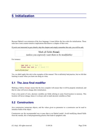
![5.3 Java initialization order
However, if you try to define an array whose size is given by a constructor parameters, the code may not
behave as you expect. Consider the following example:
The array x will always be instanciated with a size of zero ! What is happening ? If we add final modifiers
to all fields, the compiler will tell us that something is wrong:
(C) Ateji. All rights reserved. 11-09-26 Page 24/66
model MyModel solver lpsolve
{
// lower and upper are parameters of the model
double lower, upper;
// their values are given in the constructor
MyModel(double lower, double upper)
{
this.lower = lower;
this.upper = upper;
}
var double x in lower .. upper;
}
parameter-passing via a constructor
model MyModel solver lpsolve
{
// size is a parameter of the model
int size;
// its value is given in the constructor
MyModel(int size)
{
this.size = size;
}
// we want an array of the given size
var double[] x[size];
}
wrong size for x !
model MyModel solver lpsolve
{
final int size;
MyModel(int size)
{
this.size = size;
}
// Error: "The blank final field size
// may not have been initialized"
final var double[] x[size];
}
with final modifiers, the compiler signals an error](https://image.slidesharecdn.com/optimjmanualv1-170223214034/85/The-OptimJ-Manual-24-320.jpg)
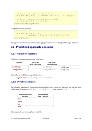
![What is happening is that Java initializes objects in this order:
1. All the fields are initialized with the blank value for their type (0 for ints, null for references, etc.)
2. The superclass is initialized
3. The fields with an inline initialization are initialized.
4. The constructor code is run
In our example, the array x is initialized first (step 3), and only then the constructor code is executed (step
4). The value of size used during the initialization of x is thus the blank value for integers, namely zero.
If size if marked final, the compiler complains that something is wrong with the initialization. It does
not complain if the final modifier is not present, and such errors are difficult to catch, this is why we
recommend to mark all fields final as much as possible. This is anyway good programming practice, as it
makes your code more understable and enables the compiler to perform some smart optimizations.
You can find all the details regarding initialization in the Java Language Specification available from
http://java.sun.com/docs/books/jls/third_edition/html/j3TOC.html
5.4 Instanciate fields in a superclass
Marking all fields final will ensure that initialization problems are caught by the compiler, but what
about the solution ?
As we have just seen, the only thing that gets executed before field initializations is the superclass
initialization (step 2). We will thus move all problematic fields into a superclass.
Our example should thus be rewritten as:
(C) Ateji. All rights reserved. 11-09-26 Page 25/66
model MyModel extends MyModelParams solver lpsolve
{
MyModel(int size)
{
// first initialize the superclass
super(size);
}
// the field size from the superclass is visible here,
// with its correct initialized value
final var double[] x[size];
}
class MyModelParams
{
// field size has been moved to the superclass
final int size;
MyModelParams(int size)
{
this.size = size;
}
}
problematic field moved into a superclass](https://image.slidesharecdn.com/optimjmanualv1-170223214034/85/The-OptimJ-Manual-25-320.jpg)
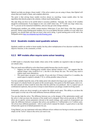
![6 Data modeling and bulk processing
Solving an optimization problem almost always involves a data processing phase before running the solver,
in order to bring the data sources in a shape suitable for modeling.
OptimJ provides another way to store information: associative arrays.
OptimJ additionally provides tuples, since it is a very common form of data : in fact, tables in relational
databases are sets of tuples.
OptimJ provides collections and aggregate operations that allow clean and concise code for bulk data
processing.
6.1 Associative arrays
Associative arrays provide another way to store information, somewhere between maps and classical Java
arrays. They behave exactly like Java arrays, but indices range over any given collection rather than over
integers from 0 to n.
The indices must be given at array creation time and can never change (unlike a Map). Even if the
collection used for defining the indices is modified later, the indices will not change.
Associative arrays are convenient for expressing optimization models in a concise mathematical-like
fashion.
6.1.1 Associative array types
An associative array type is written by writing the type of the values followed by the type of the indices
between brackets.
Here int is the type of the values, and String the type of the indices. Associative arrays can also be
multidimentional:
(C) Ateji. All rights reserved. 11-09-26 Page 26/66
int[String] myAssociativeArray;
associative array types
int[Month][Product] quantities;
multi-dimensional associative arrays](https://image.slidesharecdn.com/optimjmanualv1-170223214034/85/The-OptimJ-Manual-26-320.jpg)
![Associative and "classical" dimensions can be mixed freely. The following is an 3-dimensional array whose
first index is associative (ranging over strings), the second index is classical (ranging over 0-based
integers), and the third index is associative (ranging over booleans):
6.1.2 Creating associative arrays
Both the keys and the values must be provided when creating an associative array. A specific initializer
notation provides a convenient way to define associative arrays in-line:
The initializer notation can also be used for multidimensional arrays:
The new operator for classical arrays extends straightforwardly to associative arrays. The following
instanciates an associative arrays whose indices are taken from the collection names, and all values are
initialized to the default value of the value type (0 in this case):
The generalized declarations syntax also applies to associative arrays:
6.1.3 Accessing associative arrays
The main operation defined on associative arrays is access to a value by a key:
(C) Ateji. All rights reserved. 11-09-26 Page 27/66
int[String] ages =
{ "Stephan" -> 37,
"Lynda" -> 29 };
associative array initialization
int[String][][boolean] myAssociativeArray;
mixing associative and classical dimensions
int[String] ages = new int[names];
associative array initialisation with default values
String[] names = {"Yoann", "Bill"}; // a collection of strings
int[String] lengths[String name : names] = name.length();
// lengths = { "Yoann" -> 5, "Bill" -> 4 };
associative array creation
int[Month][Product] quantities =
{ car -> {january -> 12, february -> 17},
motorbike -> {february -> 3, october -> 37} };
multi-dimensional associative array initialization](https://image.slidesharecdn.com/optimjmanualv1-170223214034/85/The-OptimJ-Manual-27-320.jpg)
![You can iterate over all values as follows:
The field keys gives the array of indices that was used at array creation time:
Two other interesting operations exist: to know the number of keys present in an array, use field length. To
check whether an array contains a key, use method containsKey.
6.1.4 Pitfalls and usage patterns
Exactly like classical Java arrays, the types and the index values are written in reverse order:
Like for classical Java arrays, it is quite common to forget what is the proper order of indices. With
associative arrays, you can rely on the type-checker to guess what is the proper order:
Note that an associative array whith indices ranging over a integer Range is not the same as a Java array.
(C) Ateji. All rights reserved. 11-09-26 Page 28/66
ages["Stephan"] // evaluates to 37
quantities[car][january] // evaluates to 12
associative array access
for(int age: ages)... // iterate over all values
// int is the base type
// int[Month] is an array of int indexed by Month
// int[Month][Product] is an array of int[Month]
// indexed by Product
int[Month][Product] quantities = ...;
// thus when you index the array quantities, you must provide
// first the Product, then the Month
quantities[motorbike][february]
indices types and values appear in reverse order
quantities[february][motorbike] // type error
indices types and values appear in reverse order
for(String name: ages.keys)... // iterate over all keys
ages.length // 2
ages.containsKey("Lynda") // true
ages.containsKey("Peter") // false](https://image.slidesharecdn.com/optimjmanualv1-170223214034/85/The-OptimJ-Manual-28-320.jpg)
![Associative arrays do incur a space overhead compared to classical Java arrays, with a factor of
approximately 2 (for reference value types) or 4 (for primitive value types). Do not attempt to optimize
your code too early: the additional type checking provided by associative arrays is helpful for catching
common coding errors.
6.2 Tuples
OptimJ provides a notion of tuples similar to the one used in mathematics. Tuples are Java objects, with a
specific tuple type.
6.2.1 Tuple types
A tuple type is written by enumerating the types of its components between two tuple markers. Here is a
tuple type containing an integer and a string :
6.2.2 Tuple values
A similar notation is used for creating tuple values, with the keyword new :
The only operation defined on tuples is access to a component by position :
(C) Ateji. All rights reserved. 11-09-26 Page 29/66
(: int, String :) myTuple;
tuple types
myTuple = new (: 3, "Three" :);
tuple values
int[Integer] a1[int i : 0 .. 9] = i;
// a1 ranges over 0-based integers but is not a Java array.
int[] a2[int i : 10] = i; // i ranges from 0 to 9.
// a2 is a java array.
int[Integer] a3[int i : 7 .. 13] = i;
// indexes of a3 are 7, 8, ..., 13](https://image.slidesharecdn.com/optimjmanualv1-170223214034/85/The-OptimJ-Manual-29-320.jpg)
![The position is an integer literal (it cannot be an expression).
Tuples are immutable objects : once created, the values of the components cannot be changed. This enables
OptimJ to « optimize away » tuple instantiation in many common cases.
A tuple can be seen as a class defined and instantiated on the fly, where indices replace field names.
A tuple being an object, it implements all the methods of java.lang.Object. Two tuples are
equals() if their components are equals() side by side.
6.3 Collection aggregate operations
These operations provide the OptimJ equivalent of the mathematical set comprehension notation, that you
use everytime you say something like "the set of ... such that ...". They build Java collections such as
HashSet and ArrayList.
They are based on the powerful comprehension notation, which is detailed in section 7.
This example will display:
2 4 6
2 6 4 6 4
(C) Ateji. All rights reserved. 11-09-26 Page 30/66
int i = myTuple#0; // i = 3
String s = myTuple#1; // s = "Three"
tuple access
import java.util.ArrayList;
import java.util.HashSet;
import static com.ateji.monoid.Monoids.arrayList;
import static com.ateji.monoid.Monoids.hashSet;
...
int[] a = { 1, 3, 2, 3, 2 };
HashSet<Integer> s;
ArrayList<Integer> l;
s = `hashSet(){ 2*i | int i : a };
display(s);
l = `arrayList(){ 2*i | int i : a };
display(l);
building collections with the comprehension notation](https://image.slidesharecdn.com/optimjmanualv1-170223214034/85/The-OptimJ-Manual-30-320.jpg)
![6.3.1 Use cases
Collection aggregate operations provide declarative abstractions quite similar to those used in mathematics.
They are important to make your code readable: you could always replace them by a number of loop
statements, but writing "the set of ... such that ..." carries much more meaning that writing a long sequence
of imperative statements. Another benefit of using this declarative style is that it allows the compiler to
perform high-level code optimizations.
A common problem when writing optimization models is that the input data is stored along a different
"axis" then what is required by you model. For instance, countries and their respective areas may be
provided as two arrays of same length:
On the other hand, your model may require that country names and areas are given as a list of tuples:
Transforming one representation into the other may involve about a dozen lines of not very meaningful
Java code. Using OptimJ declarative notation, this is expressed in one line in an intuitive way:
Printing the elements of countries will display:
(: Jamaica ,10991.0 :) (: Japan ,377873.0 :) (: Jordan ,89342.0 :)
Use declarative notations whenever possible: your optimization code becomes more concise, more readable
and maintainable, and is likely to be more efficient.
(C) Ateji. All rights reserved. 11-09-26 Page 31/66
import optimj.util.Range;
...
Range indices = 0 .. 2;
String[] names = { "Jamaica", "Japan", "Jordan" };
double[] areas = { 10991.0, 377873.0, 89342.0 };
country names and areas as two arrays
ArrayList<(:String,double:)> countries;
country names and areas as a list of tuples
countries =
`arrayList(){ new (: names[i], areas[i] :) | int i : indices };
transforming a couple of arrays into a list of couples](https://image.slidesharecdn.com/optimjmanualv1-170223214034/85/The-OptimJ-Manual-31-320.jpg)
![6.4 Sparse data
Often, when working with large models, the data for the model tends not to be dense. Sparse data typically
involves multiple dimensions, but does not necessarily contain values for every combination of the indices.
Many storage formats (or data structures) have been proposed to represent sparse matrices. Most of them
have a Java API and can be used with OptimJ.
We will focus on solutions using associative arrays and tuples. This allows to easily skip certain
combinations of indices, that are not valid, by omitting them in the array.
6.4.1 Problem description
Consider the declaration:
transp is a two-dimensional associative array. It may represent the units shipped from a wharehouse to a
customer. But a wharehouse delivers only to a subset of customers. Array transp may be sparse.
We will present two ways to exploit the sparsity: tuples and non rectangular associative arrays.
6.4.2 Formulation in OptimJ with a set of tuples
Let us declare a set of tuples that only contains the revelant pairs (warehouse, customer). It is used to
defined the indices of associative array transp.
The sum of all units shipped is calculated as follow:
(C) Ateji. All rights reserved. 11-09-26 Page 32/66
Set<Warehouse> warehouses;
Set<Customer> customers;
int[Customer][Warehouse] transp[warehouses][customers];
Array transp may be sparse
Set<(:Warehouse, Customer:)> routes = ...;
int[(:Warehouse, Customer:)] transp[routes]
Asociative array indexed by a set of tuples.
sum{ transp[route] | (:Warehouse,Customer:) route : routes };
Sum of all units shipped](https://image.slidesharecdn.com/optimjmanualv1-170223214034/85/The-OptimJ-Manual-32-320.jpg)
![6.4.3 Formulation in OptimJ with non rectangular associative arrays
Another solution is to use a two-dimensional non-rectangular arrays:
This declaration specifies an associative array transp. For a given Warehouse w, indices of transp[w]
(computed by method customers) are a subset of set of all customers. transp is said to be non rectangular
since two different warehouses may be associated to different sets of customers.
The sum of units shipped from a given wharehouse w is calculated as follow:
6.5 Initialization
OptimJ extends the Java array initializer notation to all kinds of collections, tuples and objects.
Similarly, in OptimJ you can initialize collections by listing their values:
You can initialize tuples by giving their components:
The same notation can be used for any object: there must be exactly one constructor with the same number
of parameters. Suppose that you have defined MyClass with a constructor MyClass(int, double) :
(C) Ateji. All rights reserved. 11-09-26 Page 33/66
ArrayList<String> list = {"a", "b", "c"}; // any collection
collection initialization
(: int, int :) point = {3, 2};
tuple initialization
String[] array = {"a", "b", "c"}; // Java array
the Java array initializer notation
Set<Warehouse> warehouses;
Set<Customer> customers(Warehouse w) { return ...;}
int[Customer][Warehouse]
transp[Warehouse w:warehouses][customers(w)];
Non-rectangular associative array
sum{ transp[w][c] | Customer c : transp[w] };
Sum of units shipped](https://image.slidesharecdn.com/optimjmanualv1-170223214034/85/The-OptimJ-Manual-33-320.jpg)
![If no appropriate constructor exists, or if there are multiple constructors with the same number of
parameters, OptimJ will raise a type error.
The ambiguity between collection initialization and object initialization is resolved in favor of collections:
Initializers can be nested to any depth level, and can include associative arrays initializers:
Remember that initialization are only valid in declaration statements:
(C) Ateji. All rights reserved. 11-09-26 Page 34/66
MyClass c = {1, 1.9};
// is equivalent to MyClass c = new MyClass(1, 1.9);
object initialization
// List of appointments for each customer.
ArrayList<Date>[String] calendar = {
"Steve" -> {{2008, 06, 10}, {2008, 06, 14}},
"Monica" -> {{2008, 06, 11}},
// ...
};
nested initializers
ArrayList<String> list;
list = {"a", "b", "c"}; // wrong: this is an assignment,
// not an initialization
the initializer notation works only in an initialization
ArrayList<Integer> list = { 3 };
// this creates a one-element list containing the value 3
// if you want a list of length 3 with default values,
// use the explicit constructor new ArrayList<Integer>(3)
ambiguity](https://image.slidesharecdn.com/optimjmanualv1-170223214034/85/The-OptimJ-Manual-34-320.jpg)
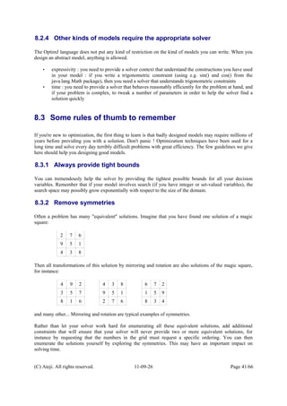
![7 Comprehensions
7.1 Comprehension expressions
We have seen the comprehension notation appearing in many different constructions of the OptimJ
language :
• in collection aggregate operations:
• in aggregate expressions:
• in aggregate constraints :
• in generalized declarations (partially) :
All these language constructs are based on the same notion of comprehension1
.
1 See for instance : Leonidas Fegaras and David Maier. Towards an Effective Calculus for Object Query
Languages. In Proceedings of the 1995 ACM SIGMOD Int'l Conference on Management of Data, May 1995.
(C) Ateji. All rights reserved. 11-09-26 Page 35/66
`hashSet(){ i | int i : 0 .. 10, :i%2==0 }
comprehension defining a collection
sum{ int i : 0 .. 10, :i%2==0 }{ i }
comprehension defining a value
var int[] a[int i : 0 .. 10] in -i .. i;
comprehension (generator only) defining an array
forall(int i : 0 .. 10, :i%2==0) {
a[i] != 0;
}
comprehension defining multiple constraints](https://image.slidesharecdn.com/optimjmanualv1-170223214034/85/The-OptimJ-Manual-35-320.jpg)
![The general form of a comprehension is either
op { target | qualifier_list }
or
op { qualifier_list } { target }
These two forms are strictly equivalent, and choosing one or the other is mainly a matter of taste and
tradition. The first one is reminiscent of the mathematical set comprehension notation (target first), while
the second is more akin to the big-Σ notation (qualifiers first).
• op is an aggregate operator (see below for a list of all predefined operators)
• target is any expression
• qualifier_list is a comma-separated list containing any number of generators and filters :
• a generator has the form type variable : expr , where
• variable is the name of the new variable introduced by the generator
• expr is an expression whose type implements the interface
java.lang.Iterable, is an array type or is an integer type.
• a filter has the form : expr , where expr is any boolean expression
Generators are used to iterate over a set of values:
Generators and filters can appear in any number and any order. For instance, these three comprehension
expressions are equivalent (as long as f does not have side effects):
The scope of the variable introduced by a generators is all generators and filters appearing to its right,
together with the target expression. A variable introduced by a generator cannot hide another local variable.
(C) Ateji. All rights reserved. 11-09-26 Page 36/66
int k;
k = sum{ int i : 10, int j : 1 .. 10, :i%2==0 }{ f(i,j) };
k = sum{ int i : 10, :i%2==0, int j : 1 .. 10 }{ f(i,j) };
k = sum{ int j : 1 .. 10, int i : 10, :i%2==0 }{ f(i,j) };
any number of generators and filters in any order
sum { k | int k in 1 .. 10} // k loops from 1 to 10
sum { k | int k in 10} // k loops from 0 to 9
sum { k | int k in new int []{3,5}} // k takes value 3 and then 5
different types of generators](https://image.slidesharecdn.com/optimjmanualv1-170223214034/85/The-OptimJ-Manual-36-320.jpg)


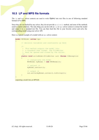
![• a*X*b, where a and b are a Java expressions and X is a decision variable
• -t or +t, where t is a constraint term
• t1 + t2, where t1 and t2 are constraint terms
• sum{ ... }{ t }, where t is a constraint term
• (t), where t is a constraint term
• a?t1:t2, where a is Java expression and t1, t2 are constraint terms
The comparisons handled by matrix-based solver contexts are boolean expressions built over terms t1 and
t2 using the following operators, where at least one of t1 or t2 involves a decision variable:
• t1 == t2
• t1 != t2
• t1 >= t2
• t1 <= t2
The following are examples of valid constraints:
The following are examples of invalid constraints:
(C) Ateji. All rights reserved. 11-09-26 Page 48/66
// a domain for String variables
String[] strings = { "abc", "def" };
// decision variables
var int I, J in 0 .. 10;
var int[] A[10] in 0 .. 10;
var double D in 0.0 .. 10.0;
var String S in strings;
// imperative variables
int i = 1;
double d = 1.0;
double f(int i, double d) { return i*d; }
constraints {
2*I + 3 == 4*J + 5;
2*(I+J) == 0;
f(i,d) * I <= 0;
f(i,d) * (I+J) >= 0;
sum{int j : 0 .. 10}{f(j,d)*A[j]} != 0;
S.charAt(0) <= 'a';
S.length() >= 4;
}
sample linear constraints](https://image.slidesharecdn.com/optimjmanualv1-170223214034/85/The-OptimJ-Manual-48-320.jpg)
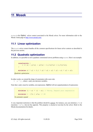
![• int sostype is the type of the SOS constraint (1 or 2).
• int priority is priority of the SOS constraint in the SOS set.
• int count is the number of variables in the SOS list.
• var int[] sosvars or var double[] sosvars or var T sosvars is an array
specifying the variables.
• double[] weights is an array specifying the count variable weights.
10.2.2 Model methods
Solving the model:
public boolean solve()
Solve the model and returns true if lp_solve has found a feasible solution.
extract() must be called before calling solve().
solve() can be called more than once. The model can be modified between calls to solve()
using the lp_solve API.
public int solverStatus()
Return detailed information about the termination of the solver (see lp_solve documentation).
Getting the solution:
public double objValue()
Returns the objective value of solution.
public public int value(var int)
public public double value(var double)
public public <T> T value(var T)
public int valueInt(var int)
public double valueDouble(var double)
public <T> T valueT(var T)
Return the solution value of the variable.
(C) Ateji. All rights reserved. 11-09-26 Page 50/66](https://image.slidesharecdn.com/optimjmanualv1-170223214034/85/The-OptimJ-Manual-50-320.jpg)

![10.3.2 Model methods
The list of methods is identical to that given above for lpsolve. The only difference concerns the solver
method :
public org.gnu.glpk.GlpkSolver solver()
10.4 Gurobi
gurobi is the OptimJ solver context associated to the Gurobi solver.OptimJ is compatible with Gurobi
versions 1 and 2. This section describes the solver context gurobi (associated to Gurobi 1.x) and
gurobi2 (associated to Gurobi 2.x). For more information refer to the Gurobi home page at
http://www.gurobi.com/.
10.4.1 Global constraints
Gurobi can handle SOS constraints written as follows:
addSOS(vars, weights, type)
where
• var int[] vars is an array specifying the variables.
• double[] weights is an array specifying the count variable weights.
• int type is the type of the SOS constraint (1 or 2).
10.4.2 Model methods
The list of methods is identical to that given above for lpsolve. The only difference concerns the acces to
the backing objects :
public gurobi.GRBModel solver()
public gurobi.GRBVar column(var int)
public gurobi.GRBVar column(var double)
public <T> gurobi.GRBVar column(var T)
public gurobi.GRBConstr row(constraints)
(C) Ateji. All rights reserved. 11-09-26 Page 52/66](https://image.slidesharecdn.com/optimjmanualv1-170223214034/85/The-OptimJ-Manual-52-320.jpg)
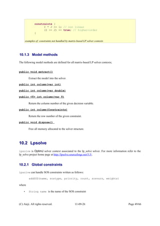
![11.3 Conic optimization
Conic optimization is a particular case of quadratic optimization that can be solve much more efficiently.
The mosek solver context can handle conic constraints written as follows:
• appendcone(conetype type, double conepar, var int[] submem)
• appendcone(conetype type, double conepar, var double[] submem)
with:
• type specifies the type of the cone. Two values are possible:
• mosek.Env.conetype.quad (quadratic cone) or
• mosek.Env.conetype.rquad (rotated quadratic cone).
• conepar: This argument is currently not used. Can be set to 0.0.
• submem: Variable subscripts of the members in the cone.
For example:
Refer to the Mosek documentation for more information about conic optimization.
11.4 Model methods
Solving the model:
public boolean solve()
Solve the model and returns true if mosek has found a feasible solution. If the problem is not
convex, a solver exception is thrown.
extract() must be called before calling solve().
solve() can be called more than once. The model can be modified between calls to solve()
using the Mosek API.
public int solverStatus()
Return detailed information about the termination of the solver (see mosek documentation).
(C) Ateji. All rights reserved. 11-09-26 Page 55/66
import mosek.Env;
constraints {
// x4 >= sqrt{x0^2 + x2^2}
mosek.appendcone(
Env.conetype.quad, // quadratic cone
0.0,
new var double []{x[4],x[0],x[2]}
);
}
Conic optimization](https://image.slidesharecdn.com/optimjmanualv1-170223214034/85/The-OptimJ-Manual-55-320.jpg)


![The following are examples of valid constraints for cplex9:
The following are examples of constraints that are not valid for cplex9:
12.1.3 CPLEX-specific constraints
(C) Ateji. All rights reserved. 11-09-26 Page 59/66
// a domain for String variables
String[] strings = { "abc", "def" };
// decision variables
var int I, J in 0 .. 10;
var int[] A[10] in 0 .. 10;
var double D in 0.0 .. 10.0;
var String S in strings;
// imperative variables
int[] a = new int [10];
int i = 1;
double d = 1.0;
double f(int i, double d) { return i*d; }
constraints {
2*I + 3 == 4*J + 5;
(I+J) * 2 == 0;
f(i,d) * I <= 0;
f(i,d) * (I+J) >= 0;
sum{int j : 0 .. 10}{f(j,d)*A[j]} == 0;
I * J >= 1; // quadratic constraint
S.charAt(0) <= 'a';
S.length() >= 4;
}
valid cplex9 constraints
constraints {
(I >= J) | (I == 5); // higher-order
I != J;
}
invalid cplex9 constraints.](https://image.slidesharecdn.com/optimjmanualv1-170223214034/85/The-OptimJ-Manual-59-320.jpg)
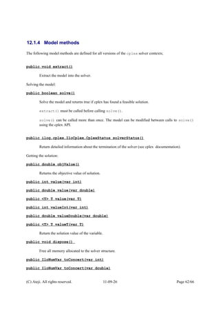
![The so-called global constraints of CPLEX can be used directly within an OptimJ constraints block
by prefixing them with the name of the solver context. All global constraints presented here apply to
cplex10 and cplex11. Refer to the CPLEX documentation for the precise meaning of these constraints.
Square:
• square(e) where e is in S10/S11.
scalar product:
• scalProd(vals, vars)
• scalProd(vals, vars,start,num)
where
• vars is an array containing the variables the scalar product.
• start is the index of the first element to use in vals and vars.
• num is the number of elements to use in vals and vars.
special ordered sets
A special ordered set (SOS) constraint basically states that among a given collection of variables, only one
variable (SOS of type 1) or only two consecutive variables (SOS of type 2) can be non-zero in any solution.
Refer to the CPLEX documentation for details.
• SOS1(vars, vals)
• SOS1(vals, vars)
• SOS1(vars, vals, start, num)
(C) Ateji. All rights reserved. 11-09-26 Page 60/66
model M solver cplex11
{
var int I in 0 .. 10, J in 5 .. 15;
constraints {
cplex11.square(I + J) >= 10; // (I+J)*(I+J) >= 10
}
}
square
model M solver cplex11
{
var int [] A [10] in -5 .. 5;
int[] a = new int [10];
constraints {
cplex11.scalProd(a,A) == 0; // a[0]*A[0]+...+a[9]*A[9]==0
cplex11.scalProd(a,A,5,3) == 0; // A[5]*a[5]+...+A[7]*a[7]==0
}
}
scalProd.](https://image.slidesharecdn.com/optimjmanualv1-170223214034/85/The-OptimJ-Manual-60-320.jpg)
![• SOS1(vals, vars, start, num)
• SOS2(vars, vals)
• SOS2(vals, vars)
• SOS2(vars, vals, start, num)
• SOS2(vals, vars, start, num)
where
• vars - An array containing the variables in the new SOS.
• vals - An array containing the weight values for the variables in the new SOS.
• start - The first element in var and val to use for the new SOS.
• num - The number of elements in var and val to use for the new SOS.
Example:
piecewise linear function :
• piecewiseLinear(expr,points,slopes,a, fa)
• piecewiseLinear(e,points,startPoints,num,slopes,startSlopes,a,fa)
where
• expr - An expression indicating where to evaluate the piecewise linear function.
• points - An array containing breakpoints that define the piecewise linear function.
• startPoints - An integer indicating the first element in array points to use for the
definition of the breakpoints of the piecewise linear function.
• num - The number of breakpoints to use from the array points. Thus num+1 elements of
array slopes are used.
• slopes - An array containing the slopes that define the piecewise linear function.
• startSlopes - The first element in array slopes to use for the definition of the slopes
of the piecewise linear function.
• a - The first coordinate of the anchor point of the piecewise linear function.
• fa - The second coordinate of the anchor point of the piecewise linear function.
(C) Ateji. All rights reserved. 11-09-26 Page 61/66
model M solver cplex11
{
var int [] sosVars [10] in -5 .. 5;
double [] weights = new double [10];
constraints {
cplex11.SOS1(sosVars, weights);
}
}
Special Ordered Sets](https://image.slidesharecdn.com/optimjmanualv1-170223214034/85/The-OptimJ-Manual-61-320.jpg)

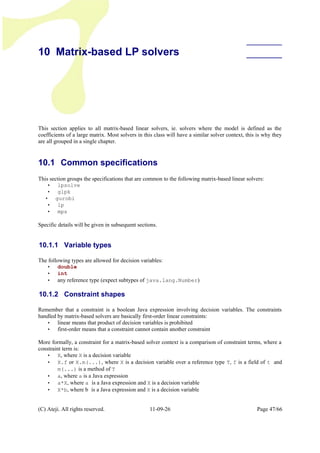
![12.2.1 Constraint shapes
Let S10 be set of OptimJ expressions that are valid constraints for cplex10. S10 is defined recursively as
follows:
• If e belongs to S9 then e belongs to S10.
• java.lang.Math.abs(e) where e belongs to S10.
• java.lang.Math.min(e) where e belongs to S10.
• java.lang.Math.max(e) where e belongs to S10.
• e1 | e2, where e1 and e2 belong to S10.
• e1 & e2, where e1 and e2 belong to S10.
• or{ ... }{ e }, where e belongs to S10.
• and{ ... }{ e }, where e belongs to S10.
• min{ ... }{ e }, where e belongs to S10.
• max{ ... }{ e }, where e belongs to S10.
• e1 => e2, where e1 and e2 belongs to S10.
• e1 != e2, where e1 or e2 belongs to S10.
• !e, where e belongs to S10.
The set S11 of OptimJ expressions that are valid constraints for the cplex11 solver context is the same as
S10.
The following are examples of valid constraints for cplex10 and cplex11:
(C) Ateji. All rights reserved. 11-09-26 Page 64/66
// decision variables
var int X in 0 .. 10;
var int Y in 0 .. 10;
var int[] A[10] in 0 .. 10;
constraints {
(X == 0) | (X == 1);
(X == 0) => (Y != 0);
// if (X==0) is true then (Y!=0) must also be true
max{var int Ai : A}{Ai} != 10;
java.lang.Math.abs( X – Y) >= 5;
!(cplex10.square(X – Y) <= 3);
sum{var int Ai : A}{?(Ai == 0)} == 3;
// There exists three i s.t. Ai == 0.
}
valid cplex10/cplex11 constraints](https://image.slidesharecdn.com/optimjmanualv1-170223214034/85/The-OptimJ-Manual-64-320.jpg)