SlideShare a Scribd company logo
1 of 250
Download to read offline
PH2101
Electrodynamics
By Dr. Soumen Basu
soumen.basu@phy.nitdgp.ac.in
Text Book : Introduction to Electrodynamics, by
David J. Griffiths
Classical Electrodynamics, by J D Jakson
What is electrodynamics?
and
how does it fit into the
general scheme of physics?
It is the dynamics/mechanics of charge particles
Or
The phenomena related to the moving charge
particles
Natural phenomena are governed by the electromagnetic interaction.
It governs our man-made world as well.
It keeps the molecules together.
+
-
Stability of
Atom
Even where you do not expect it, the electromagnetic interaction
is at work.
Mechanics tells us the reaction
of a body to a force.
Forces are described by
Newtonian Mechanics
Electromagnetism is the theory of
two types of forces:
Electric force Electric field
Magnetic force Magnetic Field
Four kinds of forces - interactions
1. Strong Keeps nuclei and nucleons together.
2. Electromagnetic Most common phenomena.
3. Weak β-decay n->p+e+ν
4. Gravitational Keeps the Universe together.
Unification
electric + magnetic electromagnetic
electrodynamic + weak electroweak
electromagnetic + optic electrodynamic
Unification of 4 Fundamental
Forces
12
Electric Charge (q, Q)
1. Charge exists as +q and –q. At the same point: +q-q=0
2. Charge is conserved (locally).
3. Charge is quantized. +q =n (+e), -q = m (-e), m, n, integer
electron: –e, positron: +e, proton: +e, C-nucleus: 6(+e)
Charge conservation in the micro world:
p + e -> n (electron capture)
Macro world: q ~ 23
10 e
Quantization is unimportant. Imagine charge as some kind of jelly.
Classical Mechanics
Newton
Quantum Field Theory
Dirac, Pauli, Feynman,
Schwinger, ….
Quantum Mechanics
Bohr, Heisenberg,
Schrödinger, …
small
Special Relativity
Einstein
fast
The Field Formulation
q q
F
E
q
v = c
Light wave
In Quantum Field theory the
difference between particles
and forces becomes rather
diffuse.
Two types of quantum particles:
Fermions and Bosons.
SI-Units
Systeme Internationale
Mechanics
length: meter (m)
mass: kilogram (kg)
time: second (s)
force: newton ( )
2

 s
m
kg
N
work: joule (J = N m)
Power: watt (W = J/s)
Electromagnetism
current: ampere (A)
charge: coulomb (C = As)
voltage: volt (V )
work: (W s = V A s)
power: watt (W = V A)
The equations of EM contain
As
Vm
C
Nm
c
Am
Vs
Vm
As 9
2
2
9
0
2
0
7
0
12
0 10
9
10
9
4
1
,
1
10
4
,
10
859
.
8 







 






The law was first discovered in 1785 by
French physicist Charles-Augustin de
Coulomb
Grifith’s Example
Statue of Johann Carl Friedrich Gauss
at his Birthplace, Brunswick,
Germany
Gauss’s law
Is Gauss’s law always true for?
=
Potential in general define
Concept of Potential
=
Now if we use the final boundary condition
l
& Magnetic field
This was discovered on 21 April 1820 by
Danish physicist Hans Christian Ørsted
Continuity equation
Jean-Baptiste Biot Félix Savart
The Biot–Savart law in magnetism is named after Biot and his colleague
Félix Savart for their work in 1820
or
Field at (2) due to (1) is
Lorentz force law predict a force on (2) towards (1)
André-Marie Ampère
Field lines for E
Field lines for B
Solenoid
Straight wire
Atom in an Electric field
Even in CO2 like simple molecule ,the relation
Paramagnetism and Ferromagnetism
Motional emf
Mathematical analysis of a series LRC
circuit - bandpass filter
R
Vin
C
L
Vout
First find the total
impedance of the circuit









C
L
i
R
Z


1









C
L
i
R
R
V
V
in
out


1
C
i
C
i
ZC





1
L
i
ZL 









 
C
L
R



1
tan 1
Using a voltage divider
The phase shift goes from
90°to -90°.
Mathematical analysis of a series LRC
circuit - bandpass filter (2)
R
Vin
C
L
Vout
The magnitude of the gain, Av, is
2
2 1










C
L
R
R
V
V
A
in
out
v


Graphing for a series LRC circuit
RLC bandpass filter
0
0.2
0.4
0.6
0.8
1
1.2
0 2 4 6
Log10 Freq
Gain
LC
fpeak

2
1

Q factor for a Series LRC circuit
RLC bandpass filter
0
0.2
0.4
0.6
0.8
1
1.2
0 2 4 6
Log10 Freq
Gain
The quality factor or Q is
defined as the energy
stored divided by the
energy loss/cycle. For an
electronic bandpass it is
the peak frequency divided
by the width of the peak
or bandwidth (defined by
the frequencies where the
gain is 3 dB lower than the
maximum).
LC
R
L
f
f
Q
dB
peak



3
2
2 1
2
1









C
L
R
R


Solve
L
R
f dB 
 3
Parallel LRC circuit
Measured across the resistor, this
circuit is a notch filter, that is it
attenuates a small band of
frequencies. The bandwidth in this
case is defined by 3dB from the
lowest point on the graph.
LC
RC
f
f
Q
dB
peak



3
 
LC
L
i
R
L
C
i
R
Z 2
1
1
1
















LC
L
i
R
R
V
V
in
out
2
1 




R
Vin
C
Vou
t
2
2
2
1









LC
L
R
R
Av


LC
fvalley

2
1

Transients in a series LRC circuit - Ringing
Suppose instead of a sinusoidal source
we had a slowly varying square
waveform or a sharp turn on of
voltage. How would a LRC circuit
behave?
We can start by using
Kirchoff’s laws again.
R
Vin
C
L
Vout
C
Q
R
dt
dQ
dt
Q
d
L
C
Q
dt
dI
L
IR
V
V
V
V C
L
R









2
2
0
This is a second order differential equation that can be solve
for the general and particular solutions.
Transients in a series LRC circuit - Ringing (2)
The solutions to the quadratic above
determine the form of the solutions.
We will just state the solutions for
different value of R, L and C.
R
Vin
C
L
Vout Overdamped
:
2
1
LC
RC







damped
Critically
:
2
1
LC
RC







ed
Underdamp
:
2
1
LC
RC







0
1
1
2



LC
x
RC
x
Transients in a series LRC circuit - Ringing (3)
The last, underdamped, results in an
exponentially decaying envelope and a
sinusoidal oscillations. This ringing is
commonly observed. It can be thought of
as two parts: a loss of energy related to R
and an oscillation related to the product LC.
This not exact so lets look at the
mathematical solution.
R
Vin
C
L
Vout















RC
t
t
C
R
LC
K
t
VR
2
exp
4
1
1
cos
)
( 2
2
1
When (RC)2>>LC the cos will oscillate several times at a
frequency almost equal to the resonant frequency.
Maxwell’s
Equations
Electrodynamics before Maxwell
Production of Electromagnetic
Waves
Since a changing electric field produces a
magnetic field, and a changing magnetic field
produces an electric field, once sinusoidal
fields are created they can propagate on their
own.
These propagating fields are called
electromagnetic waves.
This page was copied from Nick Strobel's Astronomy Notes. Go to his site at
www.astronomynotes.com for the updated and corrected version.
Production of Electromagnetic
Waves
Oscillating charges will produce
electromagnetic waves:
© 2014 Pearson
Education, Inc.
Reflection and Transmission at Oblique Incidence
Suppose that a monochromatic plane wave of frequency ω
traveling in the kI direction
Reflected wave:
Transmitted wave:
All three waves have the same frequency ω
These all share the generic structure
As for the spatial terms, evidently
But Eq. can only hold if the components are separately equal, for if x = 0,
we get
We may as well orient our axes so that kI lies in the xz plane (i.e. (k1 )y = 0);
according to Eq., so too will kR and kT. Conclusion:
First Law: The incident, reflected, and transmitted wave vectors
form a plane (called the plane of incidence), which also includes the
normal to the surface (here, the z axis).
The distance it takes to reduce the amplitude by a factor of 1/e (about a third) is called
the skin depth:
If you agree to stay away from the resonances, the damping can be ignored,
and the formula for the index of refraction simplifies:
For most substances the natural frequencies wj are scattered all over the spectrum
in a rather chaotic fashion. But for transparent materials, the nearest significant
resonances typically lie in the ultraviolet, so that w < wj. In that case,
This is known as Cauchy's formula; the constant A is called the coefficient of refraction, and B
is called the coefficient of dispersion. Cauchy's equation applies reasonably well to most gases,
in the optical region.
Potentials and Fields
The Potential Formulation
Scalar and Vector Potentials
In this chapter we seek the general solution to Maxwell's
equations
How do we express the fields in terms of scalar and vector
potentials?
B remains divergence, so we can still write,
Now, these two Equations contain all the information
in Maxwell's equations.
Gauge Transformations
Coulomb Gauge and Lorentz Gauge
The Coulomb Gauge :
Poisson's equation
Advantage: the scalar potential is particularly simple to
calculate;
Disadvantage: the vector potential is very difficult to
calculate.
The coulomb gauge is suitable for the static case.
The Lorentz Gauge
0
Retarded Potentials
Incidentally, this proof applies equally well to the
advanced potentials
A few signs are changed, but the final result is unaffected. Although the
advanced potentials are entirely consistent with Maxwell's equations, they
violate the most sacred tenet in all of physics: the principle of causality.
An infinite straight wire carries the current
The wire is presumably electrically neutral, so the scalar potential is zero. Let the
wire lie along the z axis (Fig.); the retarded vector potential at point P is
Given the retarded potentials
Jefimenko's Equations
I already calculated the gradient of V ; the time derivative of A is easy:
POINT CHARGES
Lienard-Wiechert Potentials
My next project is to calculate the (retarded) potentials, V(r, t) and
A(r, t), of a point charge q that is moving on a specified trajectory
w(t) = position of q at time t.
Example
Find the potentials of a point charge moving with constant
velocity. Assume the particle passes through the origin at
time t =0.
Sol: The trajectory is: W(t) = vt
First compute the retarded time:
The Fields of a Moving Point Charge
Using the Lienard-Wiechert potentials we can calculate the
fields of a moving point charge.
Let's begin with the gradient of V:
As for the second term, product rule 4 gives
Now
by the same argument as previous slide
Putting all this back into Eq., and using the "BAC-CAB"
rule to reduce the triple cross products
Then
A similar calculation, yields
Velocity field acceleration field
Meanwhile,
We have already calculated
Calculate the electric and magnetic fields of a point
charge moving with constant velocity.
Putting a = 0
Radiation
What is Radiation?
When charges accelerate, their fields can transport energy irreversibly out to infinity-a
process we call radiation. Let us assume the source is localized near the origin; we would
like to calculate the energy it is radiating at time t0 • Imagine a gigantic sphere, out at
radius r (Fig.) The power passing through its surface is the integral of the Poynting vector:
Because electromagnetic "news" travels at the speed of light, this
energy actually left the source at the earlier time to = t – r/c, so the
power radiated is
Electric Dipole Radiation
Then for an oscillating dipole
Magnetic Dipole Radiation
Suppose now that we have a wire loop of radius b (Fig.),
around which we drive an alternating current:
The loop is uncharged, so the scalar potential is
zero. The retarded vector potential is
For a point r directly above the x axis (Fig.), A must aim in the y
direction, since the x components from symmetrically placed points
on either side of the x axis will cancel. Thus
(cos ᵠ' serves to pick out they-component of dl'). By the law of cosines,
As before, we also assume the size of the dipole is small
compared to the wavelength radiated:
Power Radiated by a Point Charge
we derived the fields of a point charge q in arbitrary motion
The first term in this Eq. is the velocity field, and the second one (with the triple
cross-product) is the acceleration field.
The Poynting vector is
However, not all of this energy flux constitutes radiation; some of it is
just field energy carried along by the particle as it moves. The radiated
energy is the stuff that, in effect, detaches itself from the charge and
propagates off to infinity. (It’s like flies breeding on a garbage truck:
Some of them hover around the truck as it makes its rounds; others fly
away and never come back.) To calculate the total power radiated by the
particle at time tr, we draw a huge sphere of radius . (Fig. 11.10),
centered at the position of the particle (at time tr ), wait the appropriate
interval
Larmor formula
Although I derived them on the assumption that v = 0
Suppose someone is firing a stream of bullets out the window of a
moving car.
The rate Nt at which the bullets strike a stationary target is not the same as
the rate Ng at which they left the gun, because of the motion of the car. In
fact, you can easily check that N g = ( 1 – v/c) Nt. if the car is moving
towards the target, and
for arbitrary directions (here v is the velocity of the car, c is that of
the bullets relative to the ground.
Relativistic Electrodynamics
Magnetism as a Relativistic Phenomenon
net current:
A point charge q traveling to the right at speed u < v
In the reference frame where q is at rest,
by the Einstein velocity addition rule, the
velocities of the positive and negative lines are
Meanwhile, a distance s away there is a point charge q traveling
to the right at speed u < v (Fig.). Because the two line charges
cancel, there is no electrical force on q in this system (S).
Because v- > v+, the Lorentz contraction of the spacing between
negative charges is more severe;
in this frame,
the wire carries a net negative charge!
How the Fields Transform
The Field Tensor
1.Electrostatics
2. Special techniques( Laplace equation)
3. Electric fields in mater
4. Magnetostatics
5. Magnetic fields in matter
6. Electrodynamics
7. Conservation laws
8. Electromagnetic waves
9. Potentials and fields
10. Radiation
11. Electrodynamics and relativity
Introduction to Electrodynamics, David J. Griffiths

More Related Content

Similar to Electrodynamics ppt.pdfgjskysudfififkfkfififididhxdifififif

Similar to Electrodynamics ppt.pdfgjskysudfififkfkfififididhxdifififif (20)

L2 electric field, dipoles
L2  electric field, dipolesL2  electric field, dipoles
L2 electric field, dipoles
 
EMF PPT_0.pdf
EMF PPT_0.pdfEMF PPT_0.pdf
EMF PPT_0.pdf
 
[Electricity and Magnetism] Electrodynamics
[Electricity and Magnetism] Electrodynamics[Electricity and Magnetism] Electrodynamics
[Electricity and Magnetism] Electrodynamics
 
Chapter16 : Electric Force and Field
Chapter16 : Electric Force and FieldChapter16 : Electric Force and Field
Chapter16 : Electric Force and Field
 
Elaborato Luca Rapacchiani
Elaborato Luca RapacchianiElaborato Luca Rapacchiani
Elaborato Luca Rapacchiani
 
C H6
C H6C H6
C H6
 
Electric Fields
Electric FieldsElectric Fields
Electric Fields
 
Hartree fock theory
Hartree fock theoryHartree fock theory
Hartree fock theory
 
Hartree fock theory
Hartree fock theoryHartree fock theory
Hartree fock theory
 
Electricity & magnetism
Electricity & magnetismElectricity & magnetism
Electricity & magnetism
 
Electricity and magnetism
Electricity and magnetism Electricity and magnetism
Electricity and magnetism
 
Chapter-1 ECF.pptx
Chapter-1 ECF.pptxChapter-1 ECF.pptx
Chapter-1 ECF.pptx
 
Lecture20 electrostatics
Lecture20 electrostaticsLecture20 electrostatics
Lecture20 electrostatics
 
Lecture 14 on Blackbody Radiation.pptx
Lecture 14 on Blackbody Radiation.pptxLecture 14 on Blackbody Radiation.pptx
Lecture 14 on Blackbody Radiation.pptx
 
electric field, (dipoles)
  electric field, (dipoles)  electric field, (dipoles)
electric field, (dipoles)
 
Section2revision
Section2revisionSection2revision
Section2revision
 
Advchemchapt7 101015115641-phpapp02
Advchemchapt7 101015115641-phpapp02Advchemchapt7 101015115641-phpapp02
Advchemchapt7 101015115641-phpapp02
 
Lecture 6 3_coulumbs_law
Lecture 6 3_coulumbs_lawLecture 6 3_coulumbs_law
Lecture 6 3_coulumbs_law
 
Ap chem unit 7
Ap chem unit 7Ap chem unit 7
Ap chem unit 7
 
Chapter 3 wave_optics
Chapter 3 wave_opticsChapter 3 wave_optics
Chapter 3 wave_optics
 

Recently uploaded

Artificial Intelligence In Microbiology by Dr. Prince C P
Artificial Intelligence In Microbiology by Dr. Prince C PArtificial Intelligence In Microbiology by Dr. Prince C P
Artificial Intelligence In Microbiology by Dr. Prince C PPRINCE C P
 
Is RISC-V ready for HPC workload? Maybe?
Is RISC-V ready for HPC workload? Maybe?Is RISC-V ready for HPC workload? Maybe?
Is RISC-V ready for HPC workload? Maybe?Patrick Diehl
 
Traditional Agroforestry System in India- Shifting Cultivation, Taungya, Home...
Traditional Agroforestry System in India- Shifting Cultivation, Taungya, Home...Traditional Agroforestry System in India- Shifting Cultivation, Taungya, Home...
Traditional Agroforestry System in India- Shifting Cultivation, Taungya, Home...jana861314
 
GFP in rDNA Technology (Biotechnology).pptx
GFP in rDNA Technology (Biotechnology).pptxGFP in rDNA Technology (Biotechnology).pptx
GFP in rDNA Technology (Biotechnology).pptxAleenaTreesaSaji
 
Analytical Profile of Coleus Forskohlii | Forskolin .pdf
Analytical Profile of Coleus Forskohlii | Forskolin .pdfAnalytical Profile of Coleus Forskohlii | Forskolin .pdf
Analytical Profile of Coleus Forskohlii | Forskolin .pdfSwapnil Therkar
 
Natural Polymer Based Nanomaterials
Natural Polymer Based NanomaterialsNatural Polymer Based Nanomaterials
Natural Polymer Based NanomaterialsAArockiyaNisha
 
Work, Energy and Power for class 10 ICSE Physics
Work, Energy and Power for class 10 ICSE PhysicsWork, Energy and Power for class 10 ICSE Physics
Work, Energy and Power for class 10 ICSE Physicsvishikhakeshava1
 
Recombinant DNA technology( Transgenic plant and animal)
Recombinant DNA technology( Transgenic plant and animal)Recombinant DNA technology( Transgenic plant and animal)
Recombinant DNA technology( Transgenic plant and animal)DHURKADEVIBASKAR
 
Scheme-of-Work-Science-Stage-4 cambridge science.docx
Scheme-of-Work-Science-Stage-4 cambridge science.docxScheme-of-Work-Science-Stage-4 cambridge science.docx
Scheme-of-Work-Science-Stage-4 cambridge science.docxyaramohamed343013
 
Genomic DNA And Complementary DNA Libraries construction.
Genomic DNA And Complementary DNA Libraries construction.Genomic DNA And Complementary DNA Libraries construction.
Genomic DNA And Complementary DNA Libraries construction.k64182334
 
Call Girls in Mayapuri Delhi 💯Call Us 🔝9953322196🔝 💯Escort.
Call Girls in Mayapuri Delhi 💯Call Us 🔝9953322196🔝 💯Escort.Call Girls in Mayapuri Delhi 💯Call Us 🔝9953322196🔝 💯Escort.
Call Girls in Mayapuri Delhi 💯Call Us 🔝9953322196🔝 💯Escort.aasikanpl
 
Module 4: Mendelian Genetics and Punnett Square
Module 4:  Mendelian Genetics and Punnett SquareModule 4:  Mendelian Genetics and Punnett Square
Module 4: Mendelian Genetics and Punnett SquareIsiahStephanRadaza
 
All-domain Anomaly Resolution Office U.S. Department of Defense (U) Case: “Eg...
All-domain Anomaly Resolution Office U.S. Department of Defense (U) Case: “Eg...All-domain Anomaly Resolution Office U.S. Department of Defense (U) Case: “Eg...
All-domain Anomaly Resolution Office U.S. Department of Defense (U) Case: “Eg...Sérgio Sacani
 
Hubble Asteroid Hunter III. Physical properties of newly found asteroids
Hubble Asteroid Hunter III. Physical properties of newly found asteroidsHubble Asteroid Hunter III. Physical properties of newly found asteroids
Hubble Asteroid Hunter III. Physical properties of newly found asteroidsSérgio Sacani
 
Call Girls in Munirka Delhi 💯Call Us 🔝9953322196🔝 💯Escort.
Call Girls in Munirka Delhi 💯Call Us 🔝9953322196🔝 💯Escort.Call Girls in Munirka Delhi 💯Call Us 🔝9953322196🔝 💯Escort.
Call Girls in Munirka Delhi 💯Call Us 🔝9953322196🔝 💯Escort.aasikanpl
 
SOLUBLE PATTERN RECOGNITION RECEPTORS.pptx
SOLUBLE PATTERN RECOGNITION RECEPTORS.pptxSOLUBLE PATTERN RECOGNITION RECEPTORS.pptx
SOLUBLE PATTERN RECOGNITION RECEPTORS.pptxkessiyaTpeter
 
Behavioral Disorder: Schizophrenia & it's Case Study.pdf
Behavioral Disorder: Schizophrenia & it's Case Study.pdfBehavioral Disorder: Schizophrenia & it's Case Study.pdf
Behavioral Disorder: Schizophrenia & it's Case Study.pdfSELF-EXPLANATORY
 
Bentham & Hooker's Classification. along with the merits and demerits of the ...
Bentham & Hooker's Classification. along with the merits and demerits of the ...Bentham & Hooker's Classification. along with the merits and demerits of the ...
Bentham & Hooker's Classification. along with the merits and demerits of the ...Nistarini College, Purulia (W.B) India
 
A relative description on Sonoporation.pdf
A relative description on Sonoporation.pdfA relative description on Sonoporation.pdf
A relative description on Sonoporation.pdfnehabiju2046
 
Luciferase in rDNA technology (biotechnology).pptx
Luciferase in rDNA technology (biotechnology).pptxLuciferase in rDNA technology (biotechnology).pptx
Luciferase in rDNA technology (biotechnology).pptxAleenaTreesaSaji
 

Recently uploaded (20)

Artificial Intelligence In Microbiology by Dr. Prince C P
Artificial Intelligence In Microbiology by Dr. Prince C PArtificial Intelligence In Microbiology by Dr. Prince C P
Artificial Intelligence In Microbiology by Dr. Prince C P
 
Is RISC-V ready for HPC workload? Maybe?
Is RISC-V ready for HPC workload? Maybe?Is RISC-V ready for HPC workload? Maybe?
Is RISC-V ready for HPC workload? Maybe?
 
Traditional Agroforestry System in India- Shifting Cultivation, Taungya, Home...
Traditional Agroforestry System in India- Shifting Cultivation, Taungya, Home...Traditional Agroforestry System in India- Shifting Cultivation, Taungya, Home...
Traditional Agroforestry System in India- Shifting Cultivation, Taungya, Home...
 
GFP in rDNA Technology (Biotechnology).pptx
GFP in rDNA Technology (Biotechnology).pptxGFP in rDNA Technology (Biotechnology).pptx
GFP in rDNA Technology (Biotechnology).pptx
 
Analytical Profile of Coleus Forskohlii | Forskolin .pdf
Analytical Profile of Coleus Forskohlii | Forskolin .pdfAnalytical Profile of Coleus Forskohlii | Forskolin .pdf
Analytical Profile of Coleus Forskohlii | Forskolin .pdf
 
Natural Polymer Based Nanomaterials
Natural Polymer Based NanomaterialsNatural Polymer Based Nanomaterials
Natural Polymer Based Nanomaterials
 
Work, Energy and Power for class 10 ICSE Physics
Work, Energy and Power for class 10 ICSE PhysicsWork, Energy and Power for class 10 ICSE Physics
Work, Energy and Power for class 10 ICSE Physics
 
Recombinant DNA technology( Transgenic plant and animal)
Recombinant DNA technology( Transgenic plant and animal)Recombinant DNA technology( Transgenic plant and animal)
Recombinant DNA technology( Transgenic plant and animal)
 
Scheme-of-Work-Science-Stage-4 cambridge science.docx
Scheme-of-Work-Science-Stage-4 cambridge science.docxScheme-of-Work-Science-Stage-4 cambridge science.docx
Scheme-of-Work-Science-Stage-4 cambridge science.docx
 
Genomic DNA And Complementary DNA Libraries construction.
Genomic DNA And Complementary DNA Libraries construction.Genomic DNA And Complementary DNA Libraries construction.
Genomic DNA And Complementary DNA Libraries construction.
 
Call Girls in Mayapuri Delhi 💯Call Us 🔝9953322196🔝 💯Escort.
Call Girls in Mayapuri Delhi 💯Call Us 🔝9953322196🔝 💯Escort.Call Girls in Mayapuri Delhi 💯Call Us 🔝9953322196🔝 💯Escort.
Call Girls in Mayapuri Delhi 💯Call Us 🔝9953322196🔝 💯Escort.
 
Module 4: Mendelian Genetics and Punnett Square
Module 4:  Mendelian Genetics and Punnett SquareModule 4:  Mendelian Genetics and Punnett Square
Module 4: Mendelian Genetics and Punnett Square
 
All-domain Anomaly Resolution Office U.S. Department of Defense (U) Case: “Eg...
All-domain Anomaly Resolution Office U.S. Department of Defense (U) Case: “Eg...All-domain Anomaly Resolution Office U.S. Department of Defense (U) Case: “Eg...
All-domain Anomaly Resolution Office U.S. Department of Defense (U) Case: “Eg...
 
Hubble Asteroid Hunter III. Physical properties of newly found asteroids
Hubble Asteroid Hunter III. Physical properties of newly found asteroidsHubble Asteroid Hunter III. Physical properties of newly found asteroids
Hubble Asteroid Hunter III. Physical properties of newly found asteroids
 
Call Girls in Munirka Delhi 💯Call Us 🔝9953322196🔝 💯Escort.
Call Girls in Munirka Delhi 💯Call Us 🔝9953322196🔝 💯Escort.Call Girls in Munirka Delhi 💯Call Us 🔝9953322196🔝 💯Escort.
Call Girls in Munirka Delhi 💯Call Us 🔝9953322196🔝 💯Escort.
 
SOLUBLE PATTERN RECOGNITION RECEPTORS.pptx
SOLUBLE PATTERN RECOGNITION RECEPTORS.pptxSOLUBLE PATTERN RECOGNITION RECEPTORS.pptx
SOLUBLE PATTERN RECOGNITION RECEPTORS.pptx
 
Behavioral Disorder: Schizophrenia & it's Case Study.pdf
Behavioral Disorder: Schizophrenia & it's Case Study.pdfBehavioral Disorder: Schizophrenia & it's Case Study.pdf
Behavioral Disorder: Schizophrenia & it's Case Study.pdf
 
Bentham & Hooker's Classification. along with the merits and demerits of the ...
Bentham & Hooker's Classification. along with the merits and demerits of the ...Bentham & Hooker's Classification. along with the merits and demerits of the ...
Bentham & Hooker's Classification. along with the merits and demerits of the ...
 
A relative description on Sonoporation.pdf
A relative description on Sonoporation.pdfA relative description on Sonoporation.pdf
A relative description on Sonoporation.pdf
 
Luciferase in rDNA technology (biotechnology).pptx
Luciferase in rDNA technology (biotechnology).pptxLuciferase in rDNA technology (biotechnology).pptx
Luciferase in rDNA technology (biotechnology).pptx
 

Electrodynamics ppt.pdfgjskysudfififkfkfififididhxdifififif

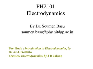
  • 1. PH2101 Electrodynamics By Dr. Soumen Basu soumen.basu@phy.nitdgp.ac.in Text Book : Introduction to Electrodynamics, by David J. Griffiths Classical Electrodynamics, by J D Jakson
  • 2. What is electrodynamics? and how does it fit into the general scheme of physics? It is the dynamics/mechanics of charge particles Or The phenomena related to the moving charge particles
  • 3. Natural phenomena are governed by the electromagnetic interaction.
  • 4.
  • 5. It governs our man-made world as well.
  • 6.
  • 7. It keeps the molecules together. + - Stability of Atom
  • 8. Even where you do not expect it, the electromagnetic interaction is at work.
  • 9. Mechanics tells us the reaction of a body to a force. Forces are described by Newtonian Mechanics
  • 10. Electromagnetism is the theory of two types of forces: Electric force Electric field Magnetic force Magnetic Field
  • 11. Four kinds of forces - interactions 1. Strong Keeps nuclei and nucleons together. 2. Electromagnetic Most common phenomena. 3. Weak β-decay n->p+e+ν 4. Gravitational Keeps the Universe together. Unification electric + magnetic electromagnetic electrodynamic + weak electroweak electromagnetic + optic electrodynamic
  • 12. Unification of 4 Fundamental Forces 12
  • 13. Electric Charge (q, Q) 1. Charge exists as +q and –q. At the same point: +q-q=0 2. Charge is conserved (locally). 3. Charge is quantized. +q =n (+e), -q = m (-e), m, n, integer electron: –e, positron: +e, proton: +e, C-nucleus: 6(+e) Charge conservation in the micro world: p + e -> n (electron capture) Macro world: q ~ 23 10 e Quantization is unimportant. Imagine charge as some kind of jelly.
  • 14. Classical Mechanics Newton Quantum Field Theory Dirac, Pauli, Feynman, Schwinger, …. Quantum Mechanics Bohr, Heisenberg, Schrödinger, … small Special Relativity Einstein fast
  • 15. The Field Formulation q q F E q v = c Light wave
  • 16. In Quantum Field theory the difference between particles and forces becomes rather diffuse. Two types of quantum particles: Fermions and Bosons.
  • 17. SI-Units Systeme Internationale Mechanics length: meter (m) mass: kilogram (kg) time: second (s) force: newton ( ) 2   s m kg N work: joule (J = N m) Power: watt (W = J/s) Electromagnetism current: ampere (A) charge: coulomb (C = As) voltage: volt (V ) work: (W s = V A s) power: watt (W = V A) The equations of EM contain As Vm C Nm c Am Vs Vm As 9 2 2 9 0 2 0 7 0 12 0 10 9 10 9 4 1 , 1 10 4 , 10 859 . 8                
  • 18. The law was first discovered in 1785 by French physicist Charles-Augustin de Coulomb
  • 19.
  • 20.
  • 21.
  • 23.
  • 24.
  • 25.
  • 26.
  • 27.
  • 28.
  • 29. Statue of Johann Carl Friedrich Gauss at his Birthplace, Brunswick, Germany Gauss’s law Is Gauss’s law always true for?
  • 30.
  • 31.
  • 32.
  • 33. = Potential in general define Concept of Potential
  • 34.
  • 35.
  • 36. =
  • 37.
  • 38.
  • 39.
  • 40.
  • 41.
  • 42.
  • 43.
  • 44.
  • 45.
  • 46.
  • 47.
  • 48.
  • 49.
  • 50.
  • 51. Now if we use the final boundary condition
  • 52.
  • 53.
  • 54.
  • 55.
  • 56.
  • 57.
  • 58.
  • 59.
  • 60.
  • 61.
  • 62. l
  • 63.
  • 64.
  • 65.
  • 66.
  • 67.
  • 68.
  • 69.
  • 70. & Magnetic field This was discovered on 21 April 1820 by Danish physicist Hans Christian Ørsted
  • 71.
  • 72. Continuity equation Jean-Baptiste Biot Félix Savart The Biot–Savart law in magnetism is named after Biot and his colleague Félix Savart for their work in 1820
  • 73. or
  • 74. Field at (2) due to (1) is Lorentz force law predict a force on (2) towards (1) André-Marie Ampère
  • 75.
  • 76.
  • 77.
  • 78.
  • 79.
  • 80. Field lines for E Field lines for B Solenoid Straight wire
  • 81.
  • 82.
  • 83.
  • 84.
  • 85. Atom in an Electric field
  • 86.
  • 87.
  • 88. Even in CO2 like simple molecule ,the relation
  • 89.
  • 90.
  • 91.
  • 92.
  • 93.
  • 94.
  • 95.
  • 96.
  • 97.
  • 98.
  • 99.
  • 100.
  • 101.
  • 102.
  • 104.
  • 105.
  • 106.
  • 107.
  • 108.
  • 109.
  • 110.
  • 112.
  • 113.
  • 114.
  • 115.
  • 116.
  • 117.
  • 118. Mathematical analysis of a series LRC circuit - bandpass filter R Vin C L Vout First find the total impedance of the circuit          C L i R Z   1          C L i R R V V in out   1 C i C i ZC      1 L i ZL             C L R    1 tan 1 Using a voltage divider The phase shift goes from 90°to -90°.
  • 119. Mathematical analysis of a series LRC circuit - bandpass filter (2) R Vin C L Vout The magnitude of the gain, Av, is 2 2 1           C L R R V V A in out v  
  • 120. Graphing for a series LRC circuit RLC bandpass filter 0 0.2 0.4 0.6 0.8 1 1.2 0 2 4 6 Log10 Freq Gain LC fpeak  2 1 
  • 121. Q factor for a Series LRC circuit RLC bandpass filter 0 0.2 0.4 0.6 0.8 1 1.2 0 2 4 6 Log10 Freq Gain The quality factor or Q is defined as the energy stored divided by the energy loss/cycle. For an electronic bandpass it is the peak frequency divided by the width of the peak or bandwidth (defined by the frequencies where the gain is 3 dB lower than the maximum). LC R L f f Q dB peak    3 2 2 1 2 1          C L R R   Solve L R f dB   3
  • 122. Parallel LRC circuit Measured across the resistor, this circuit is a notch filter, that is it attenuates a small band of frequencies. The bandwidth in this case is defined by 3dB from the lowest point on the graph. LC RC f f Q dB peak    3   LC L i R L C i R Z 2 1 1 1                 LC L i R R V V in out 2 1      R Vin C Vou t 2 2 2 1          LC L R R Av   LC fvalley  2 1 
  • 123. Transients in a series LRC circuit - Ringing Suppose instead of a sinusoidal source we had a slowly varying square waveform or a sharp turn on of voltage. How would a LRC circuit behave? We can start by using Kirchoff’s laws again. R Vin C L Vout C Q R dt dQ dt Q d L C Q dt dI L IR V V V V C L R          2 2 0 This is a second order differential equation that can be solve for the general and particular solutions.
  • 124. Transients in a series LRC circuit - Ringing (2) The solutions to the quadratic above determine the form of the solutions. We will just state the solutions for different value of R, L and C. R Vin C L Vout Overdamped : 2 1 LC RC        damped Critically : 2 1 LC RC        ed Underdamp : 2 1 LC RC        0 1 1 2    LC x RC x
  • 125. Transients in a series LRC circuit - Ringing (3) The last, underdamped, results in an exponentially decaying envelope and a sinusoidal oscillations. This ringing is commonly observed. It can be thought of as two parts: a loss of energy related to R and an oscillation related to the product LC. This not exact so lets look at the mathematical solution. R Vin C L Vout                RC t t C R LC K t VR 2 exp 4 1 1 cos ) ( 2 2 1 When (RC)2>>LC the cos will oscillate several times at a frequency almost equal to the resonant frequency.
  • 127.
  • 128.
  • 129.
  • 130.
  • 131.
  • 132.
  • 133.
  • 134.
  • 135.
  • 136.
  • 137. Production of Electromagnetic Waves Since a changing electric field produces a magnetic field, and a changing magnetic field produces an electric field, once sinusoidal fields are created they can propagate on their own. These propagating fields are called electromagnetic waves.
  • 138. This page was copied from Nick Strobel's Astronomy Notes. Go to his site at www.astronomynotes.com for the updated and corrected version.
  • 139. Production of Electromagnetic Waves Oscillating charges will produce electromagnetic waves: © 2014 Pearson Education, Inc.
  • 140.
  • 141.
  • 142.
  • 143.
  • 144.
  • 145.
  • 146.
  • 147.
  • 148.
  • 149.
  • 150.
  • 151.
  • 152.
  • 153. Reflection and Transmission at Oblique Incidence Suppose that a monochromatic plane wave of frequency ω traveling in the kI direction Reflected wave: Transmitted wave:
  • 154. All three waves have the same frequency ω These all share the generic structure As for the spatial terms, evidently
  • 155. But Eq. can only hold if the components are separately equal, for if x = 0, we get We may as well orient our axes so that kI lies in the xz plane (i.e. (k1 )y = 0); according to Eq., so too will kR and kT. Conclusion: First Law: The incident, reflected, and transmitted wave vectors form a plane (called the plane of incidence), which also includes the normal to the surface (here, the z axis).
  • 156.
  • 157.
  • 158.
  • 159.
  • 160.
  • 161.
  • 162.
  • 163.
  • 164.
  • 165.
  • 166.
  • 167. The distance it takes to reduce the amplitude by a factor of 1/e (about a third) is called the skin depth:
  • 168.
  • 169.
  • 170.
  • 171.
  • 172. If you agree to stay away from the resonances, the damping can be ignored, and the formula for the index of refraction simplifies:
  • 173. For most substances the natural frequencies wj are scattered all over the spectrum in a rather chaotic fashion. But for transparent materials, the nearest significant resonances typically lie in the ultraviolet, so that w < wj. In that case, This is known as Cauchy's formula; the constant A is called the coefficient of refraction, and B is called the coefficient of dispersion. Cauchy's equation applies reasonably well to most gases, in the optical region.
  • 174. Potentials and Fields The Potential Formulation Scalar and Vector Potentials In this chapter we seek the general solution to Maxwell's equations How do we express the fields in terms of scalar and vector potentials? B remains divergence, so we can still write,
  • 175. Now, these two Equations contain all the information in Maxwell's equations.
  • 176.
  • 178. Coulomb Gauge and Lorentz Gauge The Coulomb Gauge : Poisson's equation Advantage: the scalar potential is particularly simple to calculate;
  • 179. Disadvantage: the vector potential is very difficult to calculate. The coulomb gauge is suitable for the static case. The Lorentz Gauge 0
  • 180.
  • 181.
  • 183.
  • 184.
  • 185.
  • 186. Incidentally, this proof applies equally well to the advanced potentials A few signs are changed, but the final result is unaffected. Although the advanced potentials are entirely consistent with Maxwell's equations, they violate the most sacred tenet in all of physics: the principle of causality.
  • 187. An infinite straight wire carries the current
  • 188. The wire is presumably electrically neutral, so the scalar potential is zero. Let the wire lie along the z axis (Fig.); the retarded vector potential at point P is
  • 189.
  • 190. Given the retarded potentials Jefimenko's Equations I already calculated the gradient of V ; the time derivative of A is easy:
  • 191.
  • 192.
  • 193. POINT CHARGES Lienard-Wiechert Potentials My next project is to calculate the (retarded) potentials, V(r, t) and A(r, t), of a point charge q that is moving on a specified trajectory w(t) = position of q at time t.
  • 194.
  • 195.
  • 196. Example Find the potentials of a point charge moving with constant velocity. Assume the particle passes through the origin at time t =0. Sol: The trajectory is: W(t) = vt First compute the retarded time:
  • 197.
  • 198. The Fields of a Moving Point Charge Using the Lienard-Wiechert potentials we can calculate the fields of a moving point charge.
  • 199. Let's begin with the gradient of V: As for the second term, product rule 4 gives
  • 200. Now
  • 201. by the same argument as previous slide Putting all this back into Eq., and using the "BAC-CAB" rule to reduce the triple cross products Then
  • 202.
  • 203. A similar calculation, yields Velocity field acceleration field
  • 205. Calculate the electric and magnetic fields of a point charge moving with constant velocity. Putting a = 0
  • 206.
  • 207. Radiation What is Radiation? When charges accelerate, their fields can transport energy irreversibly out to infinity-a process we call radiation. Let us assume the source is localized near the origin; we would like to calculate the energy it is radiating at time t0 • Imagine a gigantic sphere, out at radius r (Fig.) The power passing through its surface is the integral of the Poynting vector: Because electromagnetic "news" travels at the speed of light, this energy actually left the source at the earlier time to = t – r/c, so the power radiated is
  • 209.
  • 210. Then for an oscillating dipole
  • 211.
  • 212.
  • 213.
  • 214.
  • 215. Magnetic Dipole Radiation Suppose now that we have a wire loop of radius b (Fig.), around which we drive an alternating current:
  • 216. The loop is uncharged, so the scalar potential is zero. The retarded vector potential is For a point r directly above the x axis (Fig.), A must aim in the y direction, since the x components from symmetrically placed points on either side of the x axis will cancel. Thus (cos ᵠ' serves to pick out they-component of dl'). By the law of cosines,
  • 217.
  • 218. As before, we also assume the size of the dipole is small compared to the wavelength radiated:
  • 219.
  • 220.
  • 221.
  • 222. Power Radiated by a Point Charge we derived the fields of a point charge q in arbitrary motion The first term in this Eq. is the velocity field, and the second one (with the triple cross-product) is the acceleration field. The Poynting vector is
  • 223. However, not all of this energy flux constitutes radiation; some of it is just field energy carried along by the particle as it moves. The radiated energy is the stuff that, in effect, detaches itself from the charge and propagates off to infinity. (It’s like flies breeding on a garbage truck: Some of them hover around the truck as it makes its rounds; others fly away and never come back.) To calculate the total power radiated by the particle at time tr, we draw a huge sphere of radius . (Fig. 11.10), centered at the position of the particle (at time tr ), wait the appropriate interval
  • 225. Although I derived them on the assumption that v = 0 Suppose someone is firing a stream of bullets out the window of a moving car. The rate Nt at which the bullets strike a stationary target is not the same as the rate Ng at which they left the gun, because of the motion of the car. In fact, you can easily check that N g = ( 1 – v/c) Nt. if the car is moving towards the target, and for arbitrary directions (here v is the velocity of the car, c is that of the bullets relative to the ground.
  • 226.
  • 227. Relativistic Electrodynamics Magnetism as a Relativistic Phenomenon net current: A point charge q traveling to the right at speed u < v In the reference frame where q is at rest, by the Einstein velocity addition rule, the velocities of the positive and negative lines are Meanwhile, a distance s away there is a point charge q traveling to the right at speed u < v (Fig.). Because the two line charges cancel, there is no electrical force on q in this system (S). Because v- > v+, the Lorentz contraction of the spacing between negative charges is more severe;
  • 228. in this frame, the wire carries a net negative charge!
  • 229.
  • 230. How the Fields Transform
  • 231.
  • 232.
  • 233.
  • 234.
  • 235.
  • 236.
  • 237.
  • 238.
  • 240.
  • 241.
  • 242.
  • 243.
  • 244.
  • 245.
  • 246.
  • 247.
  • 248.
  • 249.
  • 250. 1.Electrostatics 2. Special techniques( Laplace equation) 3. Electric fields in mater 4. Magnetostatics 5. Magnetic fields in matter 6. Electrodynamics 7. Conservation laws 8. Electromagnetic waves 9. Potentials and fields 10. Radiation 11. Electrodynamics and relativity Introduction to Electrodynamics, David J. Griffiths