
Recommended
More Related Content
Similar to 15 Probability Distribution Practical (HSC).pdf
Similar to 15 Probability Distribution Practical (HSC).pdf (20)
Recently uploaded
Recently uploaded (20)
15 Probability Distribution Practical (HSC).pdf
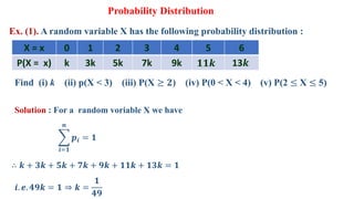
- 1. Ex. (1). A random variable X has the following probability distribution : Probability Distribution X = x 0 1 2 3 4 5 6 P(X = x) k 3k 5k 7k 9k 𝟏𝟏𝒌 13𝒌 Find (i) k (ii) p(X < 3) (iii) P(X ≥ 𝟐) (iv) P(0 < X < 4) (v) P(2 ≤ X ≤ 5) Solution : For a random voriable X we have 𝒑𝒊 = 𝟏 𝒏 𝒊=𝟏 ∴ 𝒌 + 𝟑𝒌 + 𝟓𝒌 + 𝟕𝒌 + 𝟗𝒌 + 𝟏𝟏𝒌 + 𝟏𝟑𝒌 = 𝟏 𝒊. 𝒆. 𝟒𝟗𝒌 = 𝟏 ⇒ 𝒌 = 𝟏 𝟒𝟗
- 2. X = x 0 1 2 3 4 5 6 P(X = x) 𝟏 𝟒𝟗 𝟑 𝟒𝟗 𝟓 𝟒𝟗 𝟕 𝟒𝟗 𝟗 𝟒𝟗 𝟏𝟏 𝟒𝟗 𝟏𝟑 𝟒𝟗 (𝒊)𝒌 = 𝟏 𝟒𝟗 (ii) p(X < 3) = P(X = 0) + P(X = 1) + P(X = 2) = 𝟏 𝟒𝟗 + 𝟑 𝟒𝟗 + 𝟓 𝟒𝟗 = 𝟗 𝟒𝟗 (iii) P(X ≥ 𝟐) = P(X = 2) + P(X = 3) + P(X = 4) + P(X = 5) + P(X = 6) (iv) P(0 < X < 4) = P(X = 1) + P(X = 2) + P(X = 3) (v) P(2 ≤ X ≤5) = P(X = 2) +P(X = 3) + P(X = 4) + P(X = 5) = 𝟓 𝟒𝟗 + 𝟕 𝟒𝟗 + 𝟗 𝟒𝟗 + 𝟏𝟏 𝟒𝟗 = 𝟑𝟐 𝟒𝟗
- 3. Ex. (2). Calculate the Expected value and variance of x if x denotes the number obtained on the uppermost face when o fir die is thrown. Solution : When a fair die is thrown, the sample space is S = {1,2, 3, 4, 5, 6}. The probability distribution is Let X denotes the number obtained on the upper most face. ∴ X can take values 1, 2, 3, 4, 5, 6. P(X = 1) = P(X = 2) = P(X = 3) = P(X = 4) = P(X = 5) = P(X = 6) = 𝟏 𝟔 X = x 1 2 3 4 5 6 Total P(X = x) 𝟏 𝟔 𝟏 𝟔 𝟏 𝟔 𝟏 𝟔 𝟏 𝟔 𝟏 𝟔 1
- 4. x𝒊 . p𝒊 𝟏 𝟔 𝟐 𝟔 𝟑 𝟔 𝟒 𝟔 𝟓 𝟔 𝟔 𝟔 𝟐𝟏 𝟔 = 𝟕 𝟐 𝒙𝒊 𝟐 . p𝒊 𝟏 𝟔 𝟒 𝟔 𝟗 𝟔 𝟏𝟔 𝟔 𝟐𝟓 𝟔 𝟑𝟔 𝟔 𝟗 𝟔 (i) Expected value = E(X) = 𝒙𝒊 , 𝒑𝒊 = 𝟕 𝟐 = 𝟑. 𝟓 𝒏 𝒊=𝟏 (ii) Variance = V(X) = E(𝑿𝟐) – [𝑬 𝑿 ]𝟐 𝒙𝒊 𝟐 , 𝒑𝒊 − 𝒙𝒊 , 𝒑𝒊 𝒏 𝒊=𝟏 𝟐 𝒏 𝒊=𝟏 = 𝟗𝟏 𝟔 − 𝟕 𝟐 𝟐 = 𝟗𝟏 𝟔 − 𝟒𝟗 𝟒 = 𝟏𝟖𝟐 − 𝟏𝟒𝟕 𝟏𝟐 ∴ Variance = 𝟑𝟓 𝟏𝟐 = 𝟐. 𝟗𝟏𝟔𝟕
- 5. Ex. (3). A discrete random variable X takes the values -1, 0 and 2 with the 111 probabilities 𝟏 𝟒 , 𝟏 𝟐 , 𝟏 𝟒 respectively. Find V(X) and Standard Deviation. Solution: Given that the random variable X takes the values -1, 0 and 2. The corresponding probabilities are 𝟏 𝟒 , 𝟏 𝟐 , 𝟏 𝟒 . P −𝟏 = 𝟏 𝟒 , P 𝟎 = 𝟏 𝟐 , P 𝟐 = 𝟏 𝟒 X = x -1 0 2 Total P(X = x) 𝟏 𝟒 𝟏 𝟐 𝟏 𝟒 𝟏 𝒙𝒊𝒑𝒊 - 𝟏 𝟒 𝟎 𝟏 𝟐 𝟏 𝟒 𝒙𝒊 𝟐 𝒑𝒊 𝟏 𝟒 0 1 𝟓 𝟒
- 6. (i) Variance = V(X) = E(𝑿𝟐) – [𝑬(𝑿)]𝟐 𝒙𝒊 𝟐 𝒑𝒊 − 𝒏 𝒊=𝟏 𝒙𝒊𝒑𝒊 𝒏 𝒊=𝟏 𝟐 = 𝟓 𝟒 − 𝟏 𝟒 𝟐 = 𝟓 𝟒 − 𝟏 𝟏𝟔 = 𝟓 × 𝟒 − 𝟏 𝟏𝟔 = 𝟐𝟎 − 𝟏 𝟏𝟔 = 𝟏𝟗 𝟏𝟔 = 1.1875 (ii) Standard Deviation = 𝝈 = V(X) = 𝟏𝟗 𝟏𝟔 = 𝟏. 𝟏𝟖𝟕𝟓 = 1.0897 Given data can be tabulated as follows (TABLE ON PREVIOUS PAGE )
- 7. Ex. (4). The p.d.f. of X, find P(X<1) and P( 𝑿 < 𝟏) where Solution : Given that the p.d.f of X is 𝒊 𝑷 𝑿 < 𝟏 = 𝒇 𝒙 𝒅𝒙 𝟏 −𝟐 𝒇 𝒙 = 𝒙 + 𝟐 𝟏𝟖 = 0 𝒊𝒇 − 𝟐 < 𝒙 < 𝟒 𝒐𝒕𝒉𝒆𝒓𝒘𝒊𝒔𝒆. 𝒇 𝒙 = 𝒙 + 𝟐 𝟏𝟖 = 0 𝒊𝒇 − 𝟐 < 𝒙 < 𝟒 𝒐𝒕𝒉𝒆𝒓𝒘𝒊𝒔𝒆. = 𝒙 + 𝟐 𝟏𝟖 𝒅𝒙 𝟏 −𝟐
- 8. = 𝟏 𝟏𝟖 (𝒙 + 𝟐) 𝒅𝒙 𝟏 −𝟐 = 𝟏 𝟏𝟖 (𝒙 + 𝟐)𝟐 𝟐 −𝟐 𝟏 = 𝟏 𝟑𝟔 (𝒙 + 𝟐)𝟐 −𝟐 𝟏 = 𝟏 𝟑𝟔 𝟗 − 𝟎 = 𝟗 𝟑𝟔 = 𝟗 𝟑𝟔 = 𝟎. 𝟐𝟓 (ii) P( 𝑿 < 𝟏) = P (-1 < X < 1) = 𝒙 + 𝟐 𝟏𝟖 𝒅𝒙 𝟏 −𝟏
- 9. = 𝟏 𝟏𝟖 (𝒙 + 𝟐)𝟐 𝟐 −𝟏 𝟏 = 𝟏 𝟑𝟔 (𝒙 + 𝟐)𝟐 −𝟏 𝟏 = 𝟏 𝟑𝟔 𝟗 − 𝟏 = 𝟖 𝟑𝟔 = 𝟐 𝟗 = 𝟎. 𝟐𝟐𝟐𝟐 = 𝟏 𝟏𝟖 (𝒙 + 𝟐) 𝒅𝒙 𝟏 −𝟏
- 10. Ex. (5). A random variable X has the following probability distribution : Solution: x 0 1 2 3 4 5 6 7 P(X = x) 0 k 2k 2k 3k 𝒌𝟐 2𝒌𝟐 7𝒌𝟐 + k Find (i) k (ii) (X < 3) (iii) P(X > 6) (iv) P(0 < X < 3) (v) P(2 ≤ X ≤ 4) For given probability distribution 𝒑𝒊 = 𝟏 𝒏 𝒊=𝟏 …(∵ P.D is p.m.f ) ∴ P(x = 0) + P(x = 1) + P(x = 2) + … + P(x = 7) = 1 ∴ 0 + k + 2k + 2k + 3k + 𝒌𝟐 + 2𝒌𝟐 + 7𝒌𝟐 + k = 1 ⇨ 𝟗𝒌 + 𝟏𝟎𝒌𝟐 = 𝟏
- 11. ⇨ 𝟏𝟎𝒌𝟐 + 𝟗𝒌 − 𝟏 = 𝟎 ⇨ 𝟏𝟎𝒌𝟐 + 𝟏𝟎𝒌 − 𝒌 − 𝟏 = 𝟎 ⇨ 𝟏𝟎𝒌(𝒌 + 𝟏) − 𝟏(𝒌 + 𝟏) = 𝟎 ⇨ (𝒌 + 𝟏) (10k −𝟏) = 0 ⇨ 𝒌 + 𝟏 = 0 or 10k −𝟏 = 0 𝒌 = -1 k = 𝟏 𝟏𝟎 or For 𝒌 = -1 ⇨ P.D value P 𝒙 = 𝟏 = −𝟏 which contradiction to fact 𝒑𝒊 ≥ 𝟎
- 12. ∴ 𝒌 ≠ -1 is not consider 𝐏. 𝐃. will as follows k = 𝟏 𝟏𝟎 ∴ x 0 1 2 3 4 5 6 7 P(X = x) 0 𝟏 𝟏𝟎 𝟐 𝟏𝟎 𝟐 𝟏𝟎 𝟑 𝟏𝟎 𝟏 𝟏𝟎𝟎 𝟐 𝟏𝟎𝟎 𝟏𝟕 𝟏𝟎𝟎 (ii) (X < 3) = P(x = 0 or x = 1 o r x = 2) = P(x = 0) + P(x = 1) + P(x = 2) (X < 3) = 0 + k + 2k = 3k = 𝟑 𝟏𝟎
- 13. (iii) P(X > 6) = P(x = 7) P(X > 6) = 7𝒌𝟐 + k = 𝟏𝟕 𝟏𝟎𝟎 (iv) P(0 < X < 3) = P(x = 1 or x = 2) = P(x = 1) + P(x = 2) P(0 < X < 3) = k + 2k = 3k = 𝟑 𝟏𝟎 (v) P(2 ≤ X ≤ 4) = P(x = 2 or x = 3 or x = 4) = P(x = 2) + P(x = 3) + P(x = 4) P(2 ≤ X ≤ 4) = 2k + 2k + 3k = 7k = 𝟕 𝟏𝟎
- 14. Ex. (6). The p.m.f of a random variable X is as follows : Solution: X = x 1 2 3 4 P(x) 𝟏 𝟑𝟎 𝟒 𝟑𝟎 𝟗 𝟑𝟎 𝟏𝟔 𝟑𝟎 Find Mean and Variance. 𝒙𝒊 𝒑𝒊 𝒙𝒊𝒑𝒊 𝒙𝒊 𝟐 𝒑𝒊 1 𝟏 𝟑𝟎 𝟏 𝟑𝟎 𝟏 𝟑𝟎 2 𝟏 𝟑𝟎 𝟖 𝟑𝟎 𝟏𝟔 𝟑𝟎 3 𝟗 𝟑𝟎 𝟐𝟕 𝟑𝟎 𝟖𝟏 𝟑𝟎 4 𝟏𝟔 𝟑𝟎 𝟔𝟒 𝟑𝟎 𝟐𝟓𝟔 𝟑𝟎 Total 𝒑𝒊 = 𝟏 𝒙𝒊𝒑𝒊 = 𝟏𝟎𝟎 𝟑𝟎 𝒙𝒊 𝟐 𝒑𝒊 = 𝟑𝟓𝟒 𝟑𝟎
- 15. Mean E(X) = 𝒙𝒊𝒑𝒊 = 𝟏𝟎𝟎 𝟑𝟎 𝒏 𝒊=𝟏 Mean = 𝟏𝟎𝟎 𝟑𝟎 Variance V(X) = E(𝑿𝟐 ) - [𝐄(𝐗)]𝟐 = 𝒙𝒊 𝟐 𝒑𝒊 − 𝒙𝒊𝒑𝒊 𝒏 𝒊=𝟏 𝟐 𝒏 𝒊=𝟏 = 𝟑𝟓𝟒 𝟑𝟎 − 𝟏𝟎𝟎 𝟑𝟎 𝟐 = 𝟑𝟓𝟒 𝟑𝟎 − 𝟏𝟎,𝟎𝟎𝟎 𝟗𝟎𝟎 Variance = 𝟑𝟓𝟒 ×𝟑𝟎 − 𝟏𝟎,𝟎𝟎𝟎 𝟗𝟎𝟎 = 𝟏𝟖𝟔 𝟐𝟕𝟎 = 0.6888
- 16. Ex. (7). From a survey of 20 families in a society, the following data was obtained : Solution: No. of children 0 1 2 3 4 No. of families 𝟓 𝟏𝟏 𝟐 𝟎 2 For the random variable X = number of children in a randomly chosen family, Find E(X) and V(X). Total no. families = 5 + 11 + 2 + 0 + 2 = 20 X = { 0, 1, 2, 3, 4 } Denotes random variable of no. children in a chosen family P[x = 0] = 𝟓 𝟐𝟎 P[x = 1] = 𝟏𝟏 𝟐𝟎
- 17. P[x = 2] = 𝟐 𝟐𝟎 , P[x = 3] = 𝟎 𝟐𝟎 and P[x = 4] = 𝟐 𝟐𝟎 𝒙𝒊 𝒑𝒊 𝒙𝒊𝒑𝒊 𝒙𝒊 𝟐 𝒑𝒊 0 𝟓 𝟐𝟎 𝟎 𝟎 1 𝟏𝟏 𝟐𝟎 𝟏𝟏 𝟐𝟎 𝟏𝟏 𝟐𝟎 2 𝟐 𝟐𝟎 𝟒 𝟐𝟎 𝟖 𝟐𝟎 3 𝟎 𝟐𝟎 = 0 𝟎 𝟎 4 𝟐 𝟐𝟎 𝟖 𝟐𝟎 𝟑𝟐 𝟐𝟎 Total 𝒑𝒊 = 𝟏 𝒙𝒊𝒑𝒊 = 𝟐𝟑 𝟐𝟎 𝒙𝒊 𝟐 𝒑𝒊 = 𝟓𝟏 𝟐𝟎
- 18. Mean = E(X) = 𝒙𝒊𝒑𝒊 = 𝟐𝟑 𝟐𝟎 𝒏 𝒊=𝟏 Variance = V(X) = E(𝑿𝟐) - [𝐄(𝐗)]𝟐 = 𝒙𝒊 𝟐 𝒑𝒊 − 𝒙𝒊𝒑𝒊 𝒏 𝒊=𝟏 𝟐 𝒏 𝒊=𝟏 = 𝟓𝟏 𝟐𝟎 - 𝟐𝟑 𝟐𝟎 𝟐 = 𝟓𝟏 × 𝟐𝟎 − 𝟓𝟐𝟗 𝟒𝟎𝟎 Variance = V(X) = 𝟒𝟗𝟏 𝟒𝟎𝟎 = 𝟏. 𝟐𝟐𝟕𝟓
- 19. Ex. (8). Find the c.d.f F(X) associated with the following p.d.f. f(x): Solution : 𝒇(𝒙) = 𝒇 𝒙 𝒅𝒙 𝒙 𝟎 𝒇 𝒙 = 𝟏𝟐𝒙𝟐 (𝟏 − 𝒙) = 0 𝒇𝒐𝒓 𝟎 < 𝒙 < 𝟏 𝒐𝒕𝒉𝒆𝒓𝒘𝒊𝒔𝒆. = 𝟏𝟐𝒙𝟐(𝟏 − 𝒙)𝒅𝒙 𝒙 𝟎 Also, find P 𝟏 𝟑 < 𝑿 < 𝟏 𝟐 𝒃𝒚 𝒖𝒔𝒊𝒏𝒈 𝒑. 𝒅. 𝒇 𝒂𝒏𝒅 𝒄. 𝒅. 𝒇 = 𝟏𝟐 (𝒙𝟐 − 𝒙𝟑 )𝒅𝒙 𝒙 𝟎
- 20. = 𝟏𝟐 𝒙𝟑 𝟑 − 𝒙𝟒 𝟒 𝟎 𝒙 = 𝟏𝟐 𝟒𝒙𝟑 − 𝟑𝒙𝟒 𝟏𝟐 𝒇 𝒙 = 𝟒𝒙𝟑 − 𝟑𝒙𝟒 … … . . (𝑰) 𝑵𝒐𝒘 𝑷 𝟏 𝟑 < 𝒙 < 𝟏 𝟐 𝒖𝒔𝒊𝒏𝒈 𝒑. 𝒅. 𝒇 = 𝟏𝟐𝒙𝟐(𝟏 − 𝒙)𝒅𝒙 𝟏 𝟐 𝟏 𝟑
- 21. = 𝟒𝒙𝟑 − 𝟑𝒙𝟒 𝟏 𝟑 𝟏 𝟐 = 𝟒 𝟏 𝟐 𝟑 − 𝟑 𝟏 𝟐 𝟒 − 𝟒 𝟏 𝟑 𝟑 − 𝟑 𝟏 𝟑 𝟒 = 𝟒 𝟖 − 𝟑 𝟏𝟔 − 𝟒 𝟐𝟕 − 𝟑 𝟖𝟏 = 𝟓 𝟏𝟔 − 𝟗 𝟖𝟏 = 𝟒𝟎𝟓 − 𝟏𝟒𝟒 𝟏𝟐𝟗𝟔 = 𝟐𝟗 𝟏𝟒𝟒 𝒇 𝒙 = 𝟎. 𝟐𝟎𝟏𝟑
- 22. 𝑵𝒐𝒘 𝑷 𝟏 𝟑 < 𝒙 < 𝟏 𝟐 𝒖𝒔𝒊𝒏𝒈 𝒄. 𝒅. 𝒇 𝒇 𝒙 = 𝟒𝒙𝟑 − 𝟑𝒙𝟒 = 𝒇 𝟏 𝟐 − 𝒇 𝟏 𝟑 = 𝟒 𝟏 𝟐 𝟑 − 𝟑 𝟏 𝟐 𝟒 − 𝟒 𝟏 𝟑 𝟑 − 𝟑 𝟏 𝟑 𝟒 = 𝟒 𝟖 − 𝟑 𝟏𝟔 − 𝟒 𝟐𝟕 − 𝟑 𝟖𝟏 = 𝟓 𝟏𝟔 − 𝟗 𝟖𝟏 = 𝟒𝟎𝟓 − 𝟏𝟒𝟒 𝟏𝟐𝟗𝟔
- 23. = 𝟐𝟗 𝟏𝟒𝟒 𝒇 𝒙 = 𝟎. 𝟐𝟎𝟏𝟑