An automated technique has recently been proposed to transfer learning in the hierarchical Bayesian optimization algorithm (hBOA) based on distance-based statistics. The technique enables practitioners to improve hBOA efficiency by collecting statistics from probabilistic models obtained in previous hBOA runs and using the obtained statistics to bias future hBOA runs on similar problems. The purpose of this paper is threefold: (1) test the technique on several classes of NP-complete problems, including MAXSAT, spin glasses and minimum vertex cover; (2) demonstrate that the technique is effective even when previous runs were done on problems of different size; (3) provide empirical evidence that combining transfer learning with other efficiency enhancement techniques can often yield nearly multiplicative speedups.

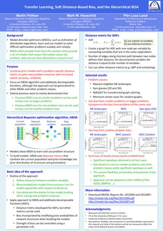
1. Transfer
Learning,
hBOA istance-­‐based
bias,
nd
based he
hierarchical
BOA
Transfer
learning,
sin d So.
for istance-­‐Based
Bias,
a and
t onierarchical
BOA
metric.
o.
D additively decomposable problems the
H a problem-specific distance However,
http://medal-lab.org
note that the framework can be applied to many other model-directed optimization techniques and the
Martin Pelikan function γ canMark W. in many other ways. To illustrate this, we outline how this approach can be
be defined Hauschild Pier Luca Lanzi
Missouri Estimation of Distribution Algorithms extended to several other model-directed optimization techniques in section 6.
Missouri Estimation of Distribution Algorithms Dipartimento di Elettronica e Informazione
Laboratory (MEDAL) Laboratory (MEDAL) Politecnico di Milano
University of Missouri, St. Louis, MO 4 Distance-Based of Missouri, St. Louis, MO
University Bias Milano, Italy
E-mail: martin@martinpelikan.net E-mail: mwh308@umsl.edu
4.1 Additively Decomposable Functions E-mail: pierluca.lanzi@polimi.it
WWW: http://martinpelikan.net/ WWW: http://www.pierlucalanzi.net/
For many optimization problems, the objective function (fitness function) can be expressed in the form of
Background
an additively decomposable function (ADF) metric
for
ADFs
Distance
of m subproblems:
• Model-­‐directed
op-mizers
(MDOs),
such
as
es#ma#on
of
• ADF
m
{Si}
are
subsets
of
variables.
3
distribu#on
algorithms,
learn
and
use
models
to
solve
f (X1 , . . . , Xn ) = fi (Si ), (5) 2.8 NK, n=50, k=5 100
with improved execution time
Multiplicative speedup w.r.t
{fi}
are
arbitrary
func-ons.
2.6 NK, n=60, k=5 90
Percentage of instances
2.4 NK, n=70, k=5
80
2.2
i=1
difficult
op-miza-on
problems
scalably
and
reliably.
2 70
CPU time
1.8 60
where (X1 , . . . , Xn ) are problem’s decision a
graph
for
ADF
with
one
node
pand ariable
b, X2 , . . . , Xn }
• Create
variables, fi is the ith subfunction, er
v Si ⊂ {X1 y
1.6 50
1.4
1.2 40
base case (no speedup)
• MDOs
o?en
provide
more
than
the
isolu-on;
they
provide
contributing to fi (subsets {Si } can overlap). Whileame
subproblem.
multiple
s the subset of variables
1 30
connec-ng
variables
that
are
in
the
s they may often exist
0.8 20
0.6 NK, n=5
0.4 10 NK, n=6
a
set
of
models
that
reveal
informa-on
about
the
0.2 0 NK, n=7
ways of decomposing the problem using additive decomposition, one would typically prefer decomposi-
• Number
of
ean example, shortest
path
between
two
nodes
for
dges
along
consider the following objective function
1 2 3 4 5 6 7 8 9 10 1 2 3 4 5 6 7
Kappa (strength of bias) Kappa (strength of
problem.
Why
not
use
that
informa#on
in
future
runs?
sizes of subsets {Si }. As
tions that minimize the
defines
their
distance;
for
disconnected
variables
the
(a) NK landscapes with neare
a problem with 6 variables:
distance
is
equal
to
the
number
of
variables.
3 2.6 SG 2D, n=144 (12x12)
3 100
with improved execution time
Multiplicative speedup w.r.t
2.8 NK, n=50, k=5 100 2.4 SG 2D, n=100 (10x10)
2.8 Kappa=10 Kappa=4
90
with improved execution time
Percentage of instances
Multiplicative speedup w.r.t
2.6 NK, n=60, k=5 90 2.2 SG 2D, n=642.6
(8x8) Kappa=8 Kappa=2
Percentage of instances
80
Average CPU speedup
NK, n=70, k=5 2 Kappa=6
Purpose
2.4 2.4
fexample (X1 , X2 , X3 , X4 , X5 , X6 ) = f1 (X1 , X2 , X5 ) + f2 (X3 , X4 ) + f3 (X2 , X5 , X6 ).
2.2
80
1.8 2.2 70
• Can
use
other
distance
metrics
(e.g.
QAP
and
scheduling).
(multiplicative)
CPU time
2 70 1.6 60
2
CPU time
1.8 60 1.4 1.8 50
1.6 50 1.2 1.6
1.4 40 SG 2D, n=144
1
• Combine
prior
models
with
a
problem-­‐specific
distance
function, there are three subsets of variables, S1 = {X1 , X2 , X5 }, S2 = {X3 , X4 } and
40 1.4 speedup)
base case (no
In the above objective 1.2
1
0.8
base case (no speedup)
30
20
0.8
0.6
1.2
1
30
20
base case (no speedup)
SG 2D, n=100 (1
SG 2D, n=
0.6 0.4
NK, n=50, k=5 0.8 10
metric
to
solve
new
problem
instances
with
,increased
three subfunctions {fesults
each of which can be defined arbitrarily.
S3 = {X2 X5 , X6 }, and 1 , f2 , f3 },
10 0.2 k=5 0.6
Selected
is not fully determined by the order (size) of subproblems, but
r
0.4 NK, n=60, 0
0.2 0 0
NK, n=70, k=5 0.4
1 2 3 4 5 6 0.2 8 9 107 1 2 3 4 5 6 7
1 2 3 4 5 6 7 8 9 10 1 2 3 4 5 6 7 8 9 10 50 55 60 65 70
It is of note that the difficulty of ADFs
speed,
accuracy,
reliability.
Kappa (strength of bias) Kappa (strength of
Kappa (strength of bias) Kappa (strength of bias) Problem size (number of bits, n)
also by the definition of the subproblems and classes:
(a) NK landscapesfact, there exist a number of NP-complete
• Problem
their interaction. In with nearest neighbors.
(b) 2D ±J Ising spin
• Focus
on
hBOA
algorithm
and
addi-vely
decomposable
problems that can be formulated as ADFs with subproblems of order 2 or 3, Speedupsas MAXSAT for 3-CNF
Figure 9: such obtained on NK landscapes and 2D
2.6
• easily define ADFs with lsubproblems of order n that can be solved
Nearest-­‐neighbor
NK
andscapes.
2.6 SG 2D, n=144 (12x12) 100 Kappa=10 Kappa=4
with improved execution time
2.4
Multiplicative speedup w.r.t
2.4 SG 2D, n=100 (10x10) Kappa=8 Kappa=2
func-ons,
although
the
approach
can
be
generalized
to
hand, one may
90
Percentage of instances
2.2
Average CPU speedup
2.2
formulas. On the other 2
SG 2D, n=64 (8x8)
80 2
Kappa=6
(multiplicative)
1.8 70 1.8
by a simple bit-flip hill climbing in low-orderglasses
(2D
time.3D).
• Spin
polynomial and
CPU time
other
MDOs
and
other
problem
classes.
1.6 60 1.6
1.4 50 1.4
1.2 1.2
40 SG 2D, n=144 (12x12)
4
1
• Extend
previous
work
to
mainly
demonstrate
that
Variable Distances • MAXSAT
for
transformed
graph
coloring.
base case (no speedup) 30 SG 2D, n=100 (10x10) 1
n=200, bias from n=150 base case n=200, bias from n=
0.8 3.5
Multiplicative speedup w.r.t
Multiplicative speedup w.r.t
0.6 20 SG 2D, n=64 (8x8) n=200, bias from n=200
3.5 0.8 (no speedup) n=200, bias from n=
4.2 Measuring for ADFs 0.4
0.2
10
0
3
0.6
0.4
3
2.5
• Previous
MDO
runs
on
smaller
problems
can
ofe
udistance between two variablesertex
cover
for
random
graphs.
based on the work
• Minimum
v of an ADF used in this paper is
CPU time
CPU time
0 2.5 0.2
The definition b a sed
1 2 3 4 5 6 7 8 9 10 1 2 3 4 5 6 7 8 9 10 64 100 144
2
Kappa (strength of bias) Kappa (strength of2bias) Problem size (number of bits, n)
1.5 1.5
to
bias
runs
on
larger
problems.
Hauschild and Pelikan (2008)• and Hauschild et smaller
problems
on
bigger
problems
Use
bias
from
al. (2012). Given an additively decomposable problem
(b) 2D ±J Ising spin glass base case (
of 1
base case (no speedup)
1
0.5 0.5
with n variables, we define the distance9: Speedups obtainedvariables using 2D graph G without using local one node per
two on NK rom
p and a spin glasses of n nodes, search.
between the
bias
flandscapesroblems
of
the
same
size)
an
two variables Xi and Xj in theo
• Previous
MDO
runs
for
one
problem
class
canybe
used
(compare
t
Figure 1 2 3 4 5 6 7 8 9 10 1 2 3 4 5 6 7
variable. For same subset Sk , that is, Xi , Xjwith nearestwe create an edgecover,G= ∈ Sk , neighbors, (b) Minimum vertex in n Kappa (strength of bias) Kappa (strength of
to
bias
runs
for
another
problem
class.
the nodes Xi and Xj . See
fig. K
for an example
of
an
M= 200, k
=
5.
Spin
glass
(2D)
N 2 landscapes
ADF and the
corresponding graph. Denoting
n VC
(a) NK landscapes
between
by li,j the number of edges along the shortest path between Xi and Xj in G (in terms of the number of
4
n=200, bias from n=150 3.5 n=200, bias from n=150
2.8
2.6
2 n=400, bias from n=324
n=200, bias from n=150
1.8
Multiplicative speedup w.r.t
Multiplicative speedup w.r.t
w.r.t
Multiplicative speedup w.r.t
Multiplicative speedup w.r.t
3.5 n=200, bias from n=200 n=200, bias from n=200 2.4 n=400, bias from n=400
n=200, bias from n=200 1.6
1.8
edges), we define the distance between two variables as 3
3 2.2
2 1.4
Hierarchical
Bayesian
opAmizaAon
algorithm,
hBOA
1.6
1.8
2.5 1.2
CPU time
CPU time
CPU time
CPU time
2.5 1.6
1.4
2 1.4 base case 1
2 1.2
1.2 (no speedup)
li,j if a path between Xi and Xj exists, and 1.5 1 base case (no speedup) 0.8
Current
Selected
Bayesian
1.5
New
0.8
1
D(Xi , Xj ) = 1 (6)
base case (no speedup)
1
base case (no speedup) 0.6 0.6
n otherwise. 0.8
0.4
popula-on
popula-on
network
0.4
popula-on
0.5 0.5 0.2
0.6
0
0.2
1 2 3 4 5 6 7 8 9 10 1 2 3 4 5 6 7 8 9 10 1 2 5 6 7 8 9 10
3 4 5 6 7 8 9 10
Kappa (strength of bias) Kappa (strength of bias) (strength of bias)
Kappa (strength of bias)
Fig. 2 illustrates the distance metric on a simple example. The above distance measure makes variables in
the same subproblem close to each Use
bias
from
another
problem
class
the distances correspond to
• other, whereas for the remaining variables,
(a) NK landscapes with nearest neighbors, (b) Minimum vertex cover, n = 200, c = 2. (d) Minimum vertex cover, n = 200, c20 = (e) 3D ±
(c) 2D ±J Ising spin glass, 20 × = 4.
n = 200, k = 5. 400 343
the length of the chain of subproblemsK
landscapes
variables.easier)
obtained on allharder)
except for
N that relate the two
MVC
Figure 10:distance
isMVC
( test problems
( The Speedups
maximal for variables
1.8
2 n=400, bias from n=324 n=343, bias from n=216
Multiplicative speedup w.r.t
Multiplicative speedup w.r.t
n=400, bias from n=400 1.6 n=343, bias from n=343
1.8
that are completely independent (the value of a variable does not from problems of smaller size, compared toof the case with
influence the contribution the base other
3
1.6
1.2
1.4
CPU time
CPU time
Models from NK 4 Models from NK Models from NK3
1.4
Multiplicative speedup w.r.t
Multiplicative speedup w.r.t
Multiplicative speedup w.r.t
2.8 Models from MVC, c=2 Models from MVC, c=2.0 Models from MVC, c=2.0
variable in any way).
2.6 Models from MVC, c=4 3.5 1
Models from MVC, c=4.0 Models from MVC, c=4.0
1.2 base case 2.5 speedup)
(no
2.4 0.8
3
base case (no speedup)
2.2 1
17 2
Since interactions between problem variables are encoded mainly in the subproblems of the additive
CPU time
CPU time
CPU time
2 2.5 0.6
1.8 0.8
1.6 2 0.4 1.5
base case
problem decomposition, the above distance metric should typically correspond closely to the likelihood 1.4
1.2 base case (no speedup)2
1
0.6
3 4 5 6 7 8
1.5 0.2
9 10 base case (no speedup) 2
1 3 4 5 6 7 8
1
9 10
(no speedup)
1 1
of dependencies between problem variables in probabilistic models discovered by EDAs. Specifically, the 0.8
0.6
Kappa (strength of bias)
0.5
Kappa (strength 0.5
of bias)
• Models
allow
hBOA
to
learn
and
use
problem
structure.
with respect to the 400
(d) 2D ±J Ising spin glass, n = 20 × 20 = (e) 3D ±J Ising spin glass, n = 7 × 7 × 7 =
0.4 0
variables located closer metric should more likely interact with each other. Fig. 3 illus-
343
1 2 3 4 5 6 7 8
Kappa (strength of bias)
9 10 1 2 3 4 5 6 7 8
Kappa (strength of bias)
9 10 1 2 3 4 5 6 7 8
Kappa (strength of bias)
9 10
trates this on two ADFs discussedNK landscapes thisnearest neighbors, (b) Minimum vertex cover, n = with 2. (c) Minimum vertex cover, n = 200, c = 4.
(a) later in with paper—the NK landscape 200, c = nearest neighbor interactions
• To
build
models,
hBOA
uses
Bayesian
metrics
that
= Summary
of
results
(many
r