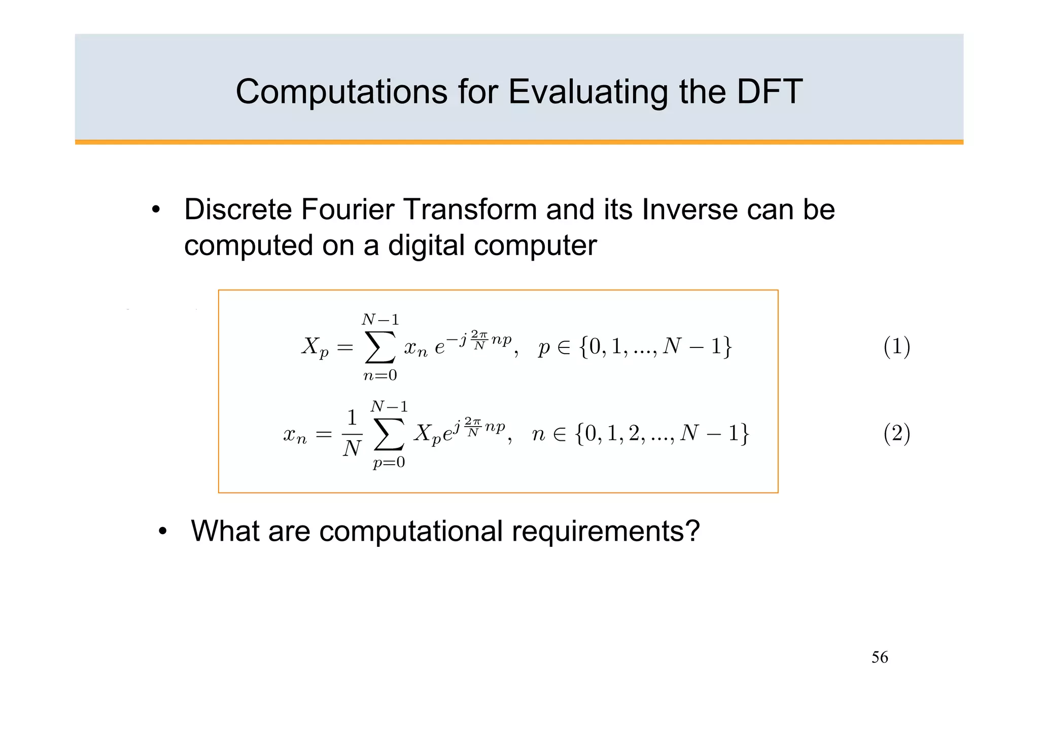
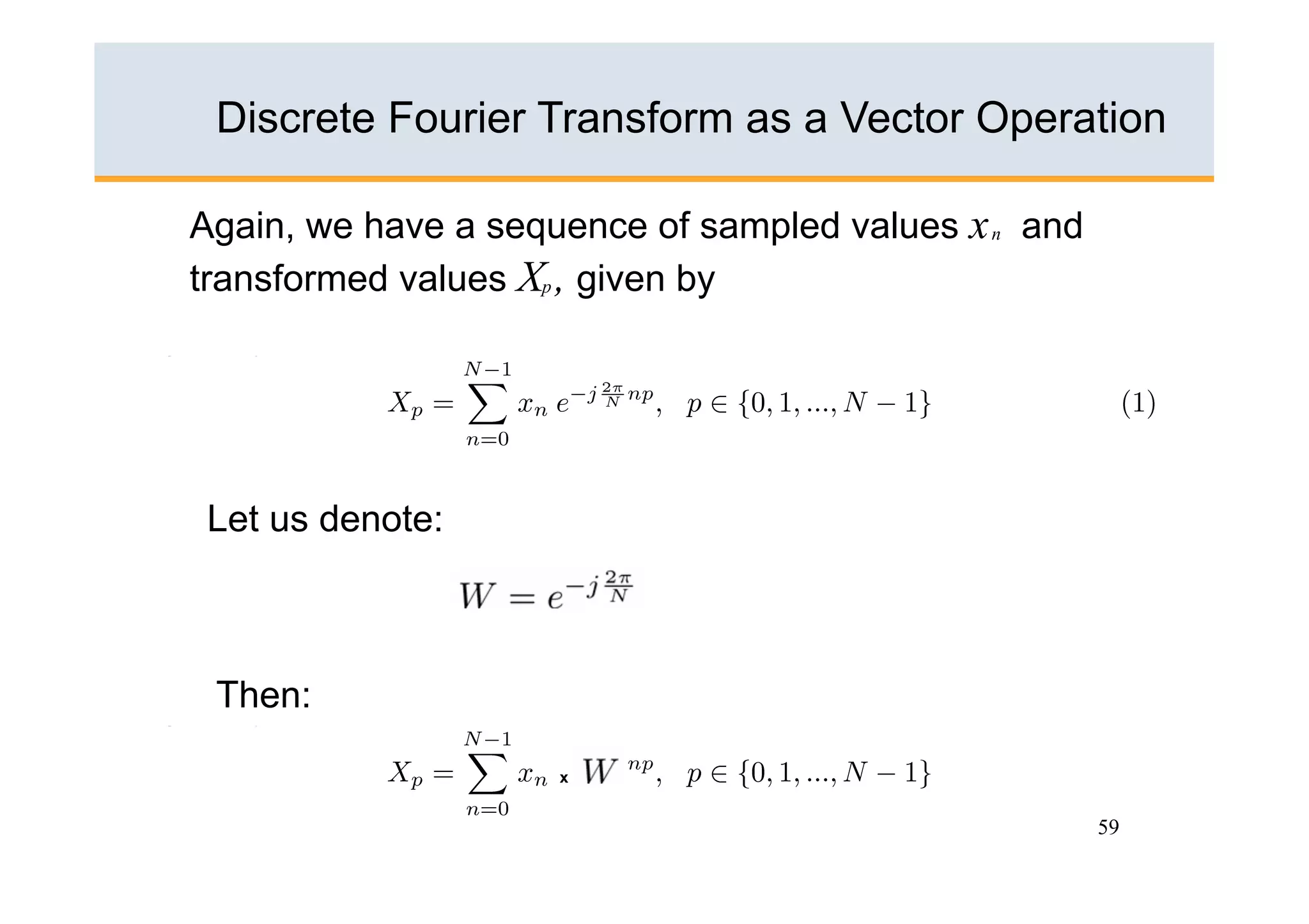
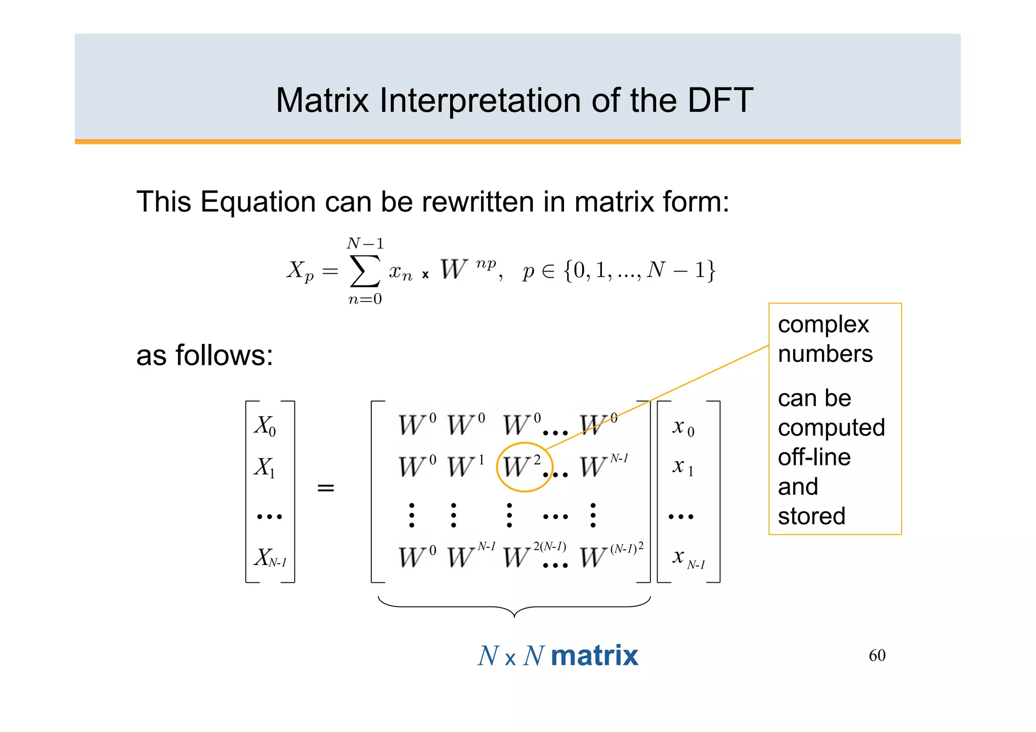
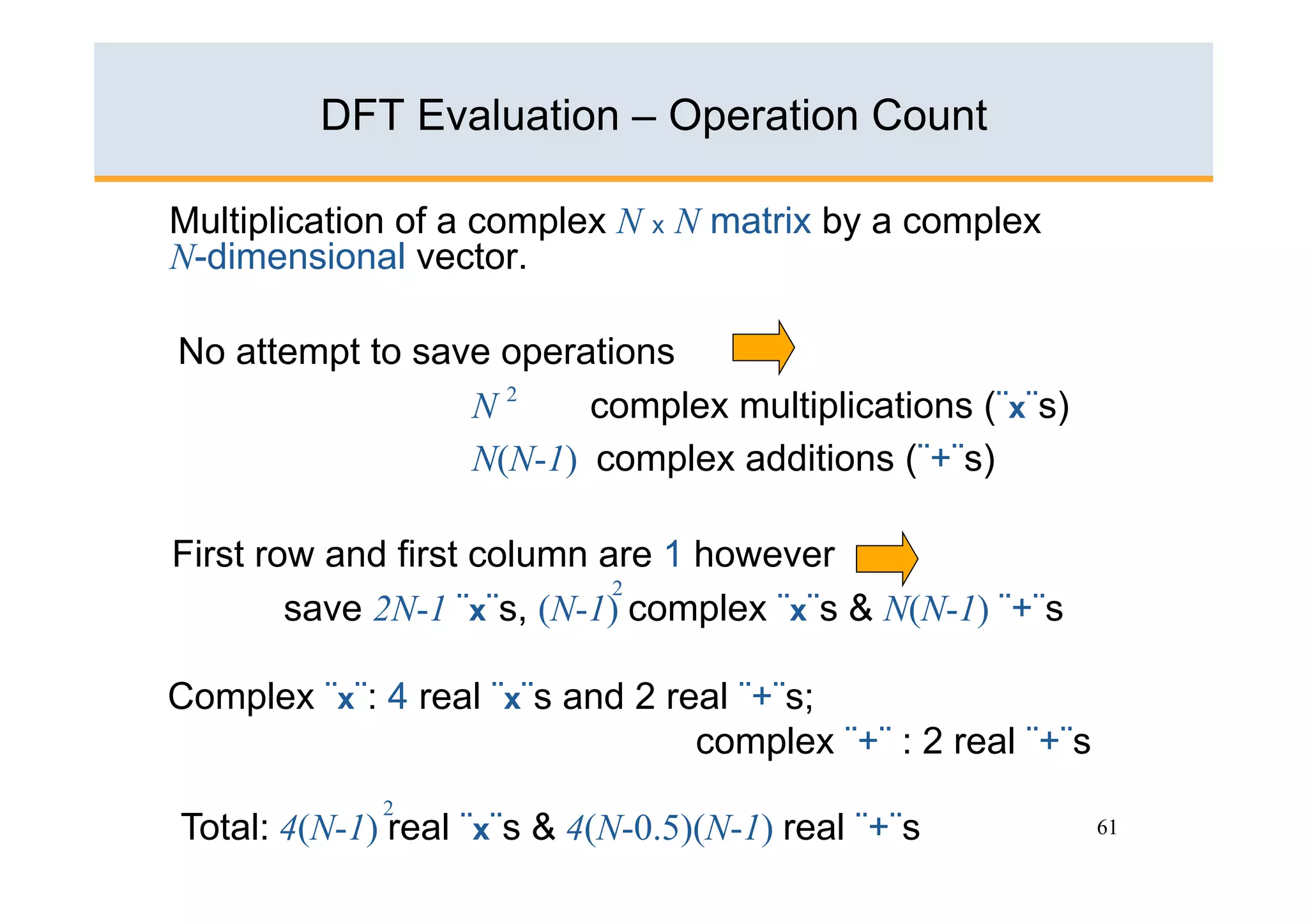
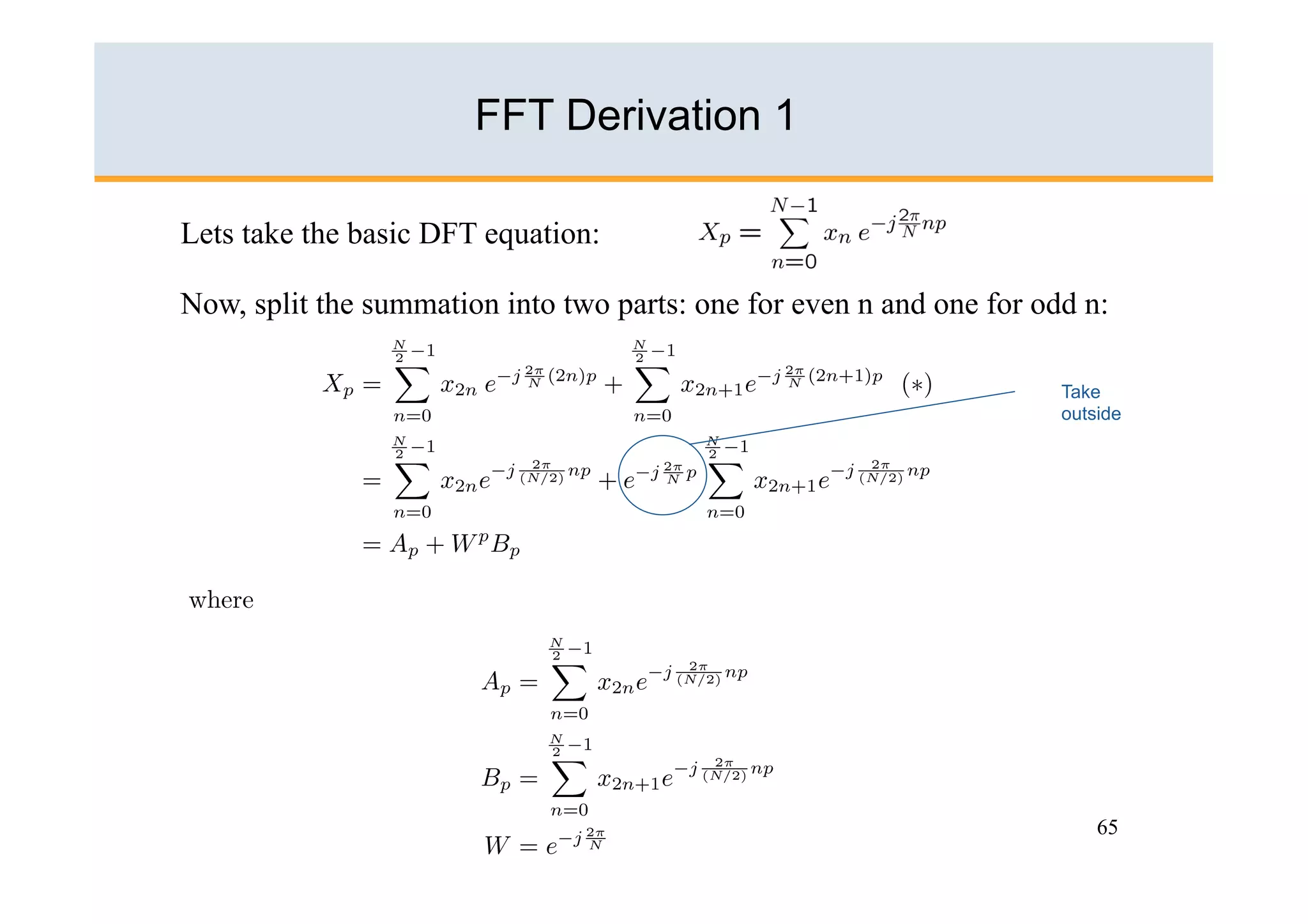
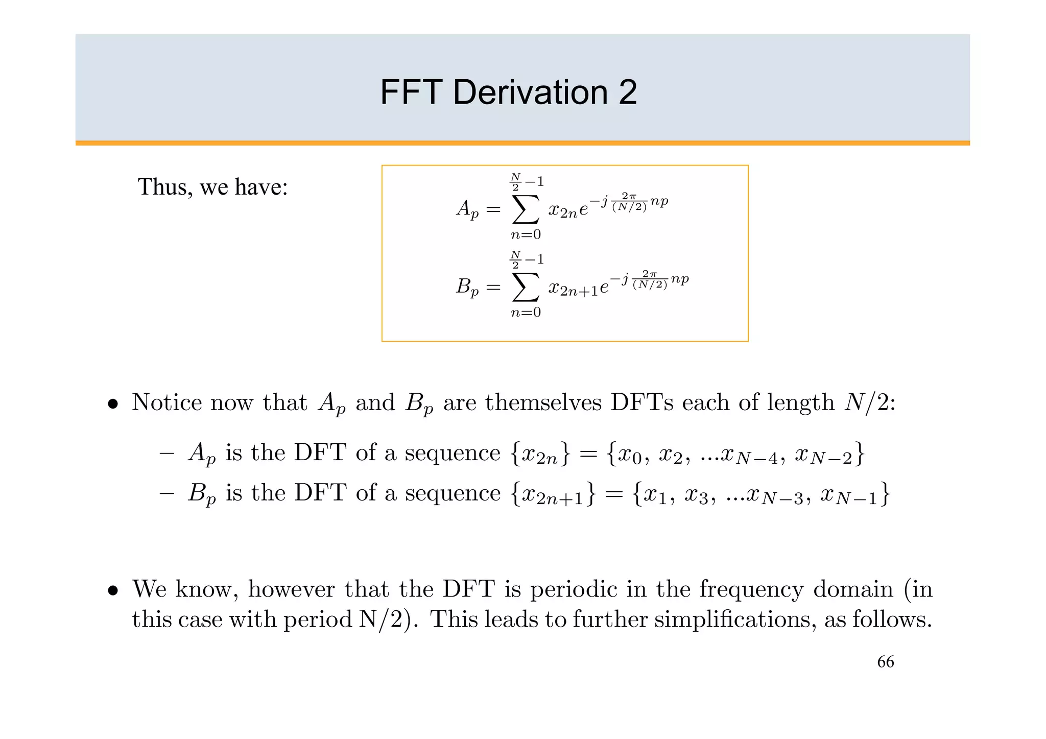
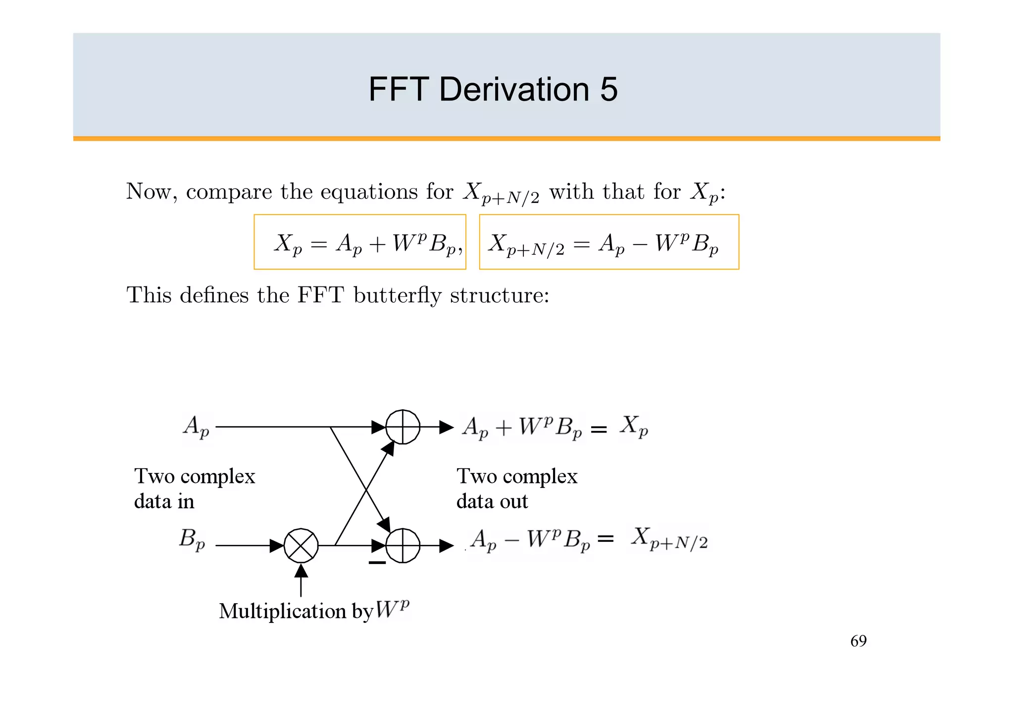
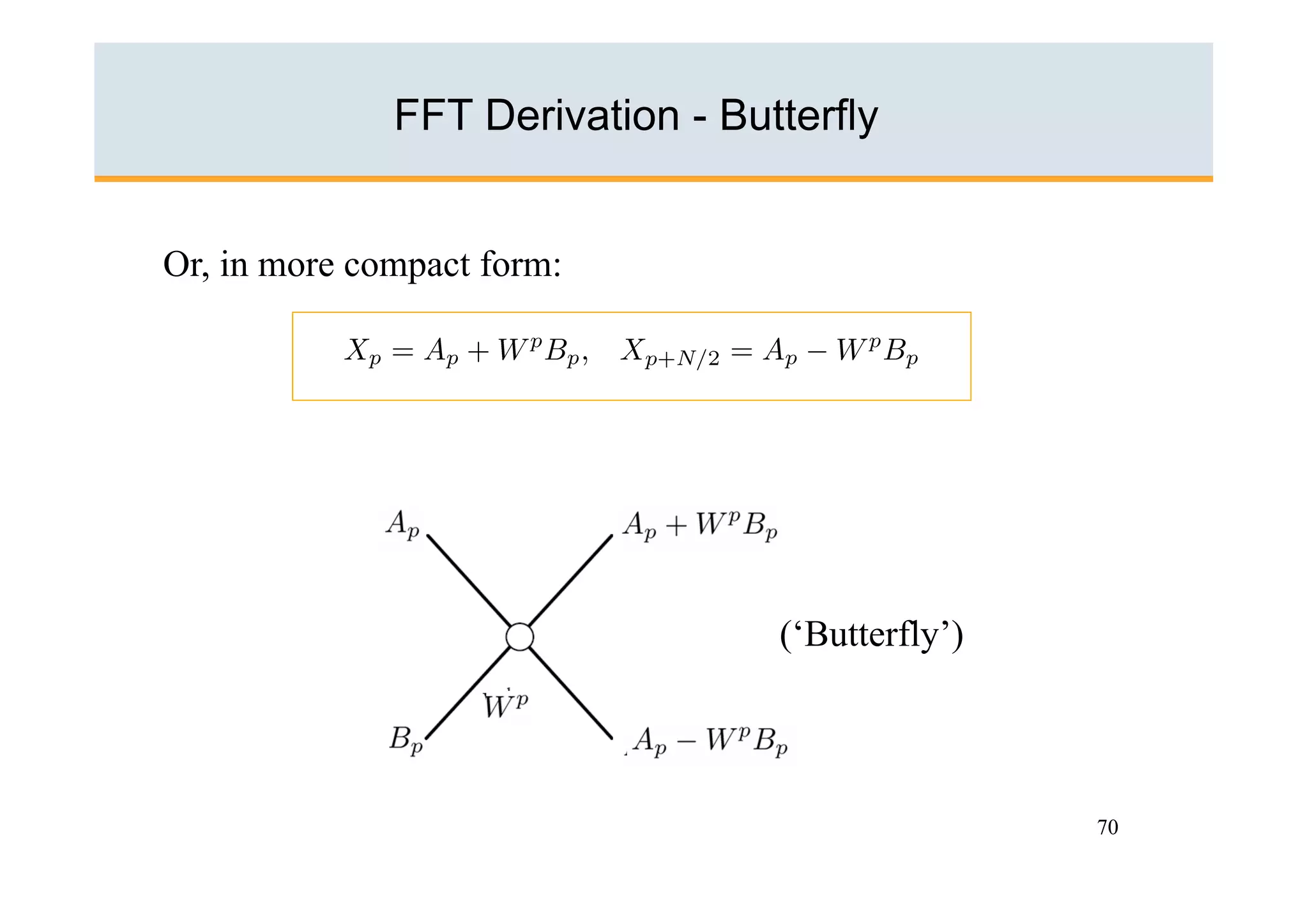
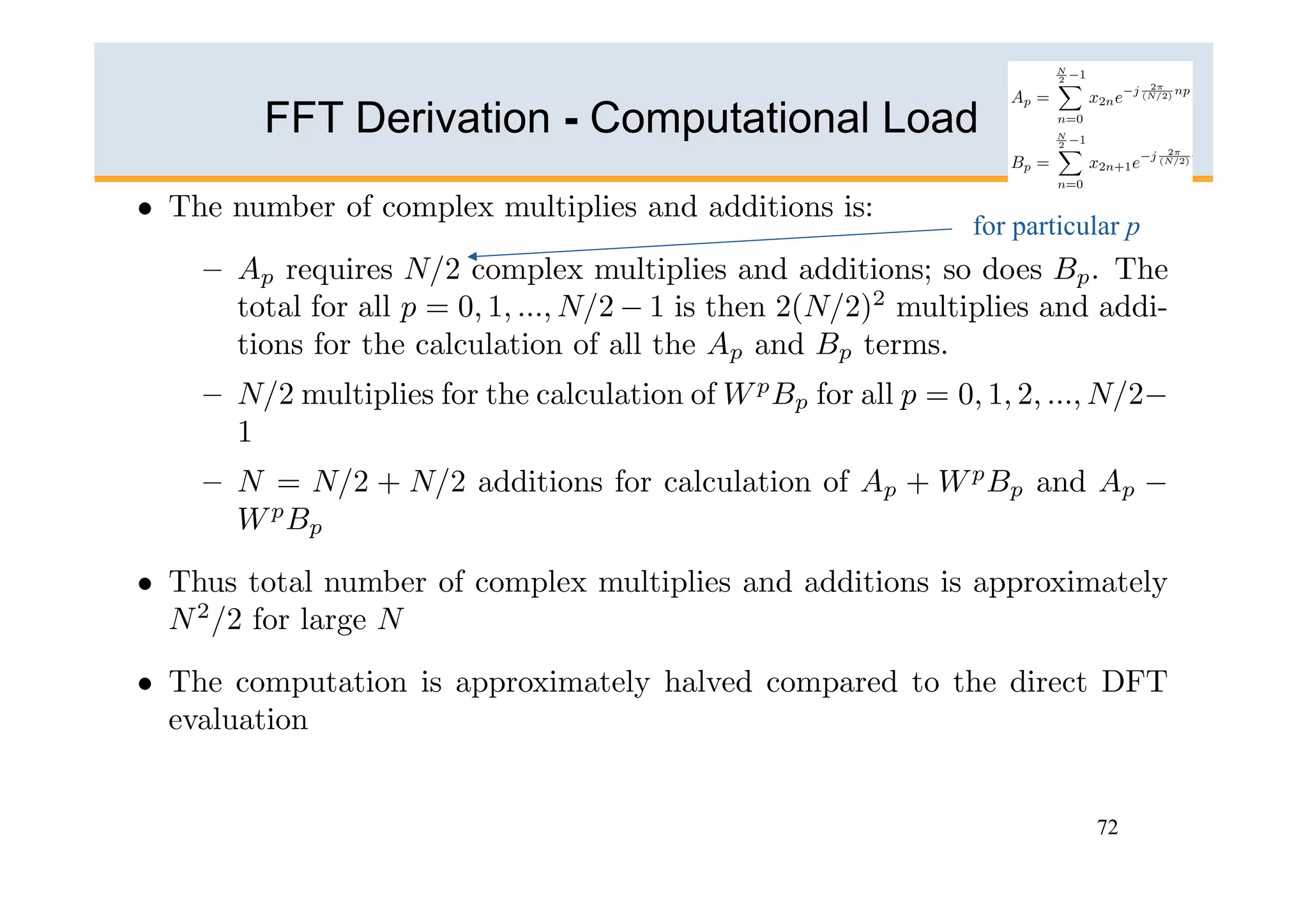
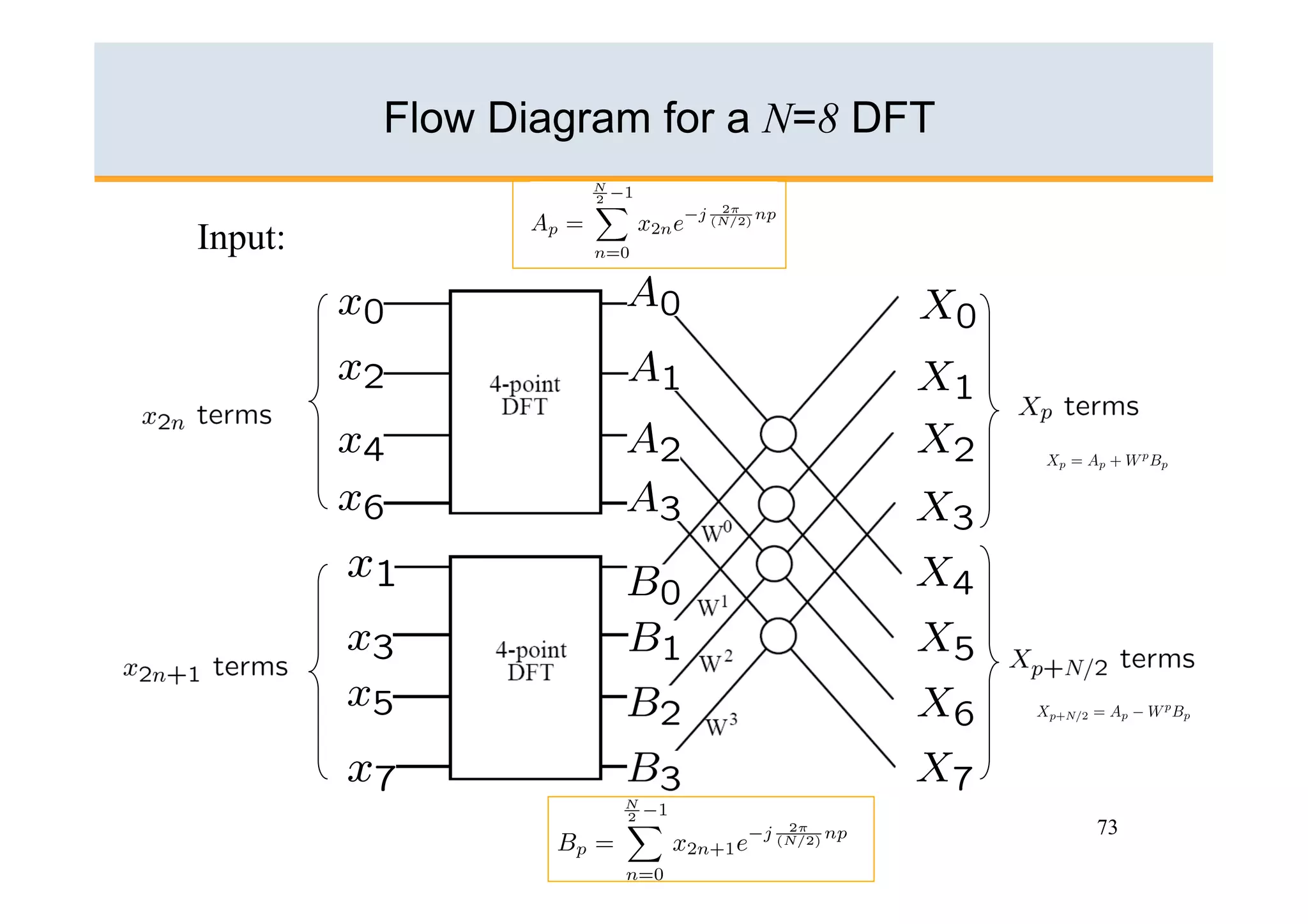
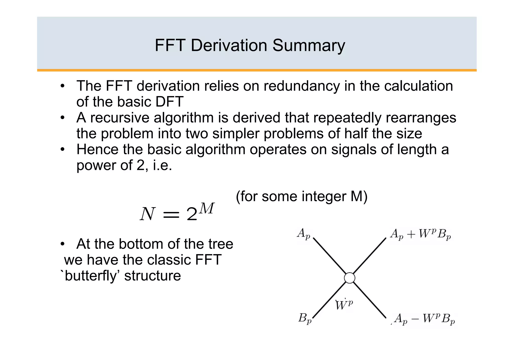
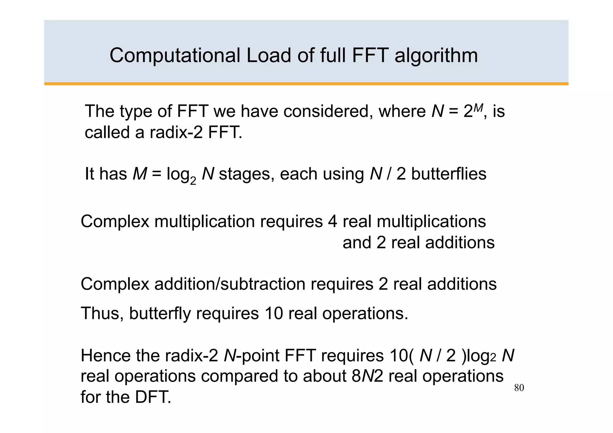
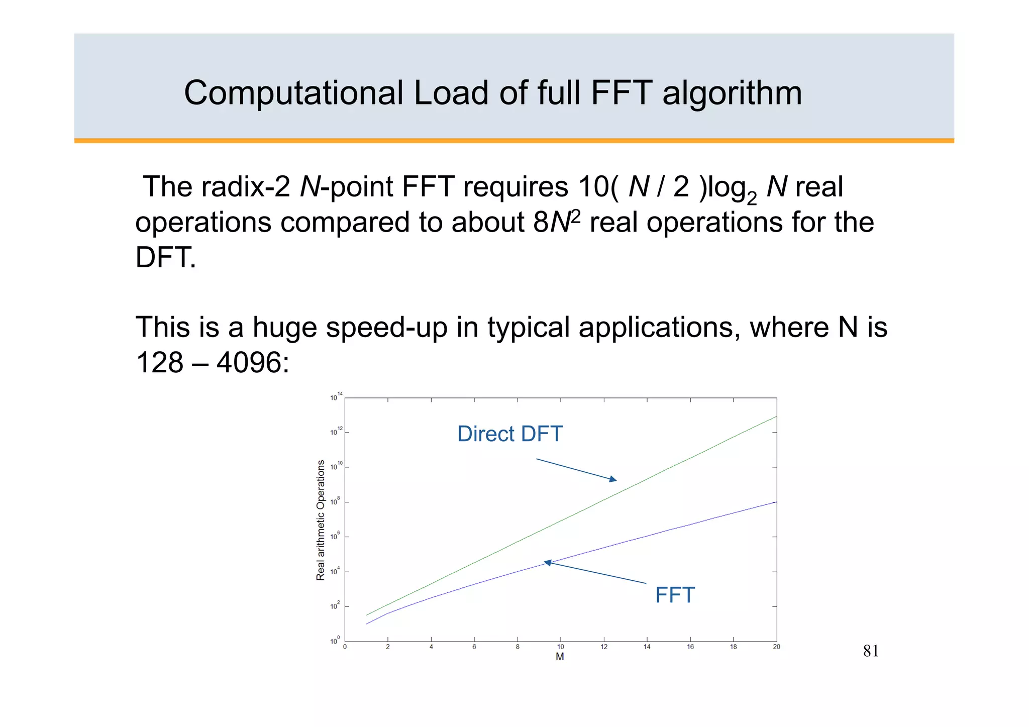
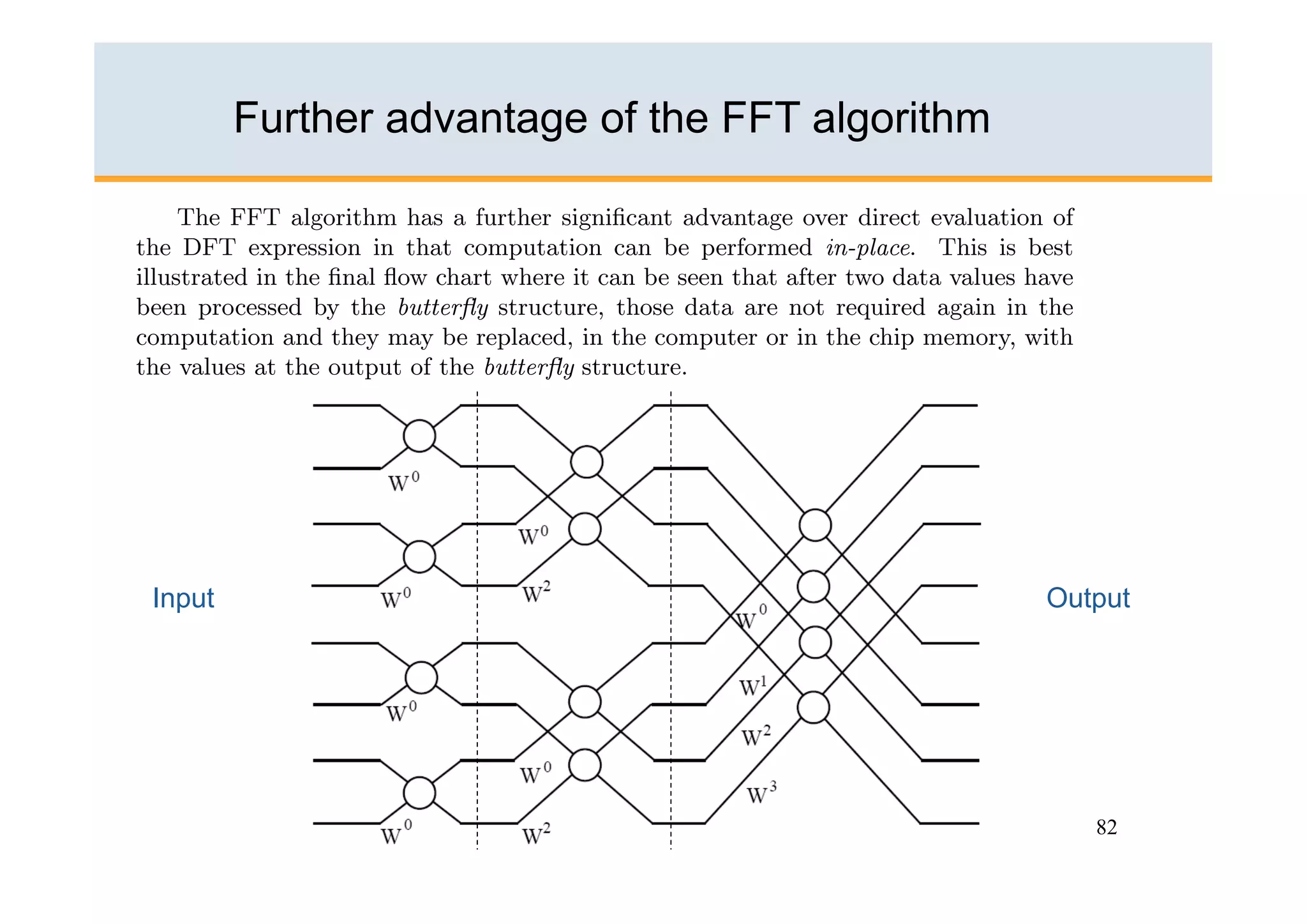
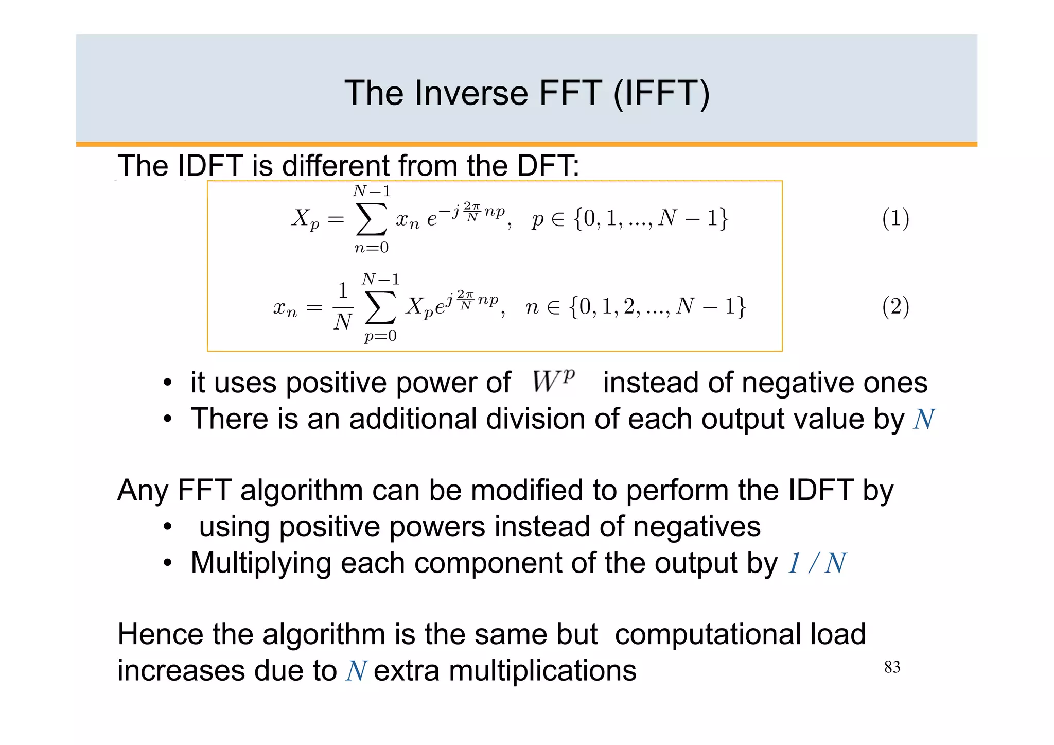
Fast Fourier Transform (FFT)


              Elena Punskaya
       www-sigproc.eng.cam.ac.uk/~op205


                                Some material adapted from courses by
                                Prof. Simon Godsill, Dr. Arnaud Doucet,
                           Dr. Malcolm Macleod and Prof. Peter Rayner


                                                                          55
Computations for Evaluating the DFT


•  Discrete Fourier Transform and its Inverse can be
   computed on a digital computer


•  What are computational requirements?


                                                       56
Operation Count

How do we evaluate computational complexity?
     count the number of real multiplications and
     additions
     by ¨real¨ we mean either fixed-point or floating point
     operations depending on the specific hardware

      subtraction is considered equivalent to additions
      divisions are counted separately

  Other operations such as loading from memory, storing in
  memory, loop counting, indexing, etc are not counted
  (depends on implementation/architecture) – present
  overhead                                             57
Operation Count – Modern DSP


Modern DSP:
     a real multiplication and addition is a single machine
     cycle y=ax+b called MAC (multiply/accumulate)

      maximum number of multiplications and additions must
      be counted, not their sum

      traditional claim ¨multiplication is much more time-
      consuming than addition¨ becomes obsolete

                                                             58
Discrete Fourier Transform as a Vector Operation

Again, we have a sequence of sampled values x n and
transformed values Xp , given by


Let us denote:


 Then:

                     x


                                                      59
Matrix Interpretation of the DFT

This Equation can be rewritten in matrix form:

                       x


                                                                complex
as follows:                                                     numbers
                                                                can be
         X0                0   0         0
                                          …   0
                                                        x0      computed
         X1                0   1         2
                                          …
                                              N-1
                                                        x1      off-line
                =                                               and
         …                                …             …
                      …
                      …
                                     …

                                              …
                                                                stored
                               N-1   2(N-1)   (N-1) 2
         XN-1              0
                                         …              x N-1


                               N x N matrix                           60
DFT Evaluation – Operation Count

Multiplication of a complex N x N matrix by a complex
N-dimensional vector.

No attempt to save operations
                 N2     complex multiplications (¨x¨s)
                 N(N-1) complex additions (¨+¨s)

First row and first column are 1 however
                            2
        save 2N-1 ¨x¨s, (N-1) complex ¨x¨s & N(N-1) ¨+¨s

Complex ¨x¨: 4 real ¨x¨s and 2 real ¨+¨s;
                                 complex ¨+¨ : 2 real ¨+¨s
             2
Total: 4(N-1) real ¨x¨s & 4(N-0.5)(N-1) real ¨+¨s            61
DFT Computational Complexity


Thus, for the input sequence of length N the number of
arithmetic operations in direct computation of DFT is
proportional to N 2
                  .

For N=1000, about a million operations are needed!


 In 1960s such a number was considered prohibitive
 in most applications.


                                                         62
Discovery of the Fast Fourier Transform (FFT)

When in 1965 Cooley and Tukey ¨first¨ announced
discovery of Fast Fourier Transform (FFT) in 1965 it
revolutionised Digital Signal Processing.


They were actually 150 years late – the principle of the
FFT was later discovered in obscure section of one of
Gauss’ (as in Gaussian) own notebooks in 1806.


Their paper is the most cited mathematical paper ever
written.

                                                           63
The Fast Fourier Transform (FFT)

The FFT is a highly elegant and efficient algorithm,
which is still one of the most used algorithms in speech
processing, communications, frequency estimation, etc
– one of the most highly developed area of DSP.

There are many different types and variations.

They are just computational schemes for computing the
DFT – not new transforms!

Here we consider the most basic radix-2 algorithm
which requires N to be a power of 2.
                                                       64
FFT Derivation 1

Lets take the basic DFT equation:

Now, split the summation into two parts: one for even n and one for odd n:

                                                                      Take
                                                                      outside


                                                                          65
FFT Derivation 2

Thus, we have:


                                    66
FFT Derivation 3

Now, take the same equation again where we split the summation
into two parts: one for even n and one for odd n:


 And evaluate at frequencies p+N/2


                                                                 67
FFT Derivation 4

                   simplified


                                68
FFT Derivation 5


              =


              =


                   69
FFT Derivation - Butterfly


Or, in more compact form:


                                  (‘Butterfly’)


                                                  70
FFT Derivation - Redundancy


                              71
FFT Derivation - Computational Load

                                  for particular p


                                             72
Flow Diagram for a N=8 DFT

Input:                       Output:


                                       73
Further decomposition

We obtained

Now
      A0, A1, A2 , A3 - N/2-point DFT

          Ap =αp +WN/2p βp         Ap+N/2 =αp -WN/2p βp

                           - using redundancy just discovered

      B0, B1, B2 , B3 - N/2-point DFT
          Bp =α /p +WN/2p β /p       Bp+N/2 =α /p -WN/2p β /p

                           - using redundancy just discovered
Finally
          WN/2p =e-j2πp/N/2=e-j2π2p/N=WN2p
                                                                74
Flow Diagram for a N=8 DFT - Decomposition


           α0
           α1
           β0
           β1
           α /0
           α /1
           β /0
           β /1                         75
Further decomposition

We obtained

Now
      A0, A1, A2 , A3 - N/2-point DFT

          Ap =αp +WN/2p βp         Ap+N/2 =αp -WN/2p βp

                           - using redundancy just discovered

      B0, B1, B2 , B3 - N/2-point DFT
          Bp =α /p +WN/2p β /p       Bp+N/2 =α /p -WN/2p β /p

                           - using redundancy just discovered
Finally
          WN/2p =e-j2πp/N/2=e-j2π2p/N=WN2p
                                                                76
Flow Diagram for a N=8 DFT – Decomposition 2


         α0
         α1
         β0

         β1
         α /0
         α /1
         β /0
         β /1
                                        77
Bit-reversal


               78
FFT Derivation Summary

•  The FFT derivation relies on redundancy in the calculation
   of the basic DFT
•  A recursive algorithm is derived that repeatedly rearranges
   the problem into two simpler problems of half the size
•  Hence the basic algorithm operates on signals of length a
   power of 2, i.e.

                               (for some integer M)


•  At the bottom of the tree
 we have the classic FFT
`butterfly’ structure


                                                          79
Computational Load of full FFT algorithm

The type of FFT we have considered, where N = 2M, is
called a radix-2 FFT.

It has M = log2 N stages, each using N / 2 butterflies

Complex multiplication requires 4 real multiplications
                                  and 2 real additions

Complex addition/subtraction requires 2 real additions
Thus, butterfly requires 10 real operations.

Hence the radix-2 N-point FFT requires 10( N / 2 )log2 N
real operations compared to about 8N2 real operations
                                                         80
for the DFT.
Computational Load of full FFT algorithm

The radix-2 N-point FFT requires 10( N / 2 )log2 N real
operations compared to about 8N2 real operations for the
DFT.

This is a huge speed-up in typical applications, where N is
128 – 4096:

                         Direct DFT


                                        FFT

                                                         81
Further advantage of the FFT algorithm


Input                                            Output


                                                    82
The Inverse FFT (IFFT)

The IDFT is different from the DFT:


   •  it uses positive power of        instead of negative ones
   •  There is an additional division of each output value by N

Any FFT algorithm can be modified to perform the IDFT by
   •  using positive powers instead of negatives
   •  Multiplying each component of the output by 1 / N

Hence the algorithm is the same but computational load
increases due to N extra multiplications                   83
Many types of FFT
The form of FFT we have described is called “decimation in time”; there
is a form called “decimation in frequency” (but it has no advantages).

The "radix 2" FFT must have length N a power of 2. Slightly more efficient
is the "radix 4" FFT, in which 2-input 2-output butterflies are replaced by 4-
input 4-output units. The transform length must then be a power of 4
(more restrictive).

A completely different type of algorithm, the Winograd Fourier Transform
Algorithm (WFTA), can be used for FFT lengths equal to the product of a
number of mutually prime factors (e.g. 9*7*5 = 315 or 5*16 = 80). The
WFTA uses fewer multipliers, but more adders, than a similar-length FFT.

Efficient algorithms exist for FFTing real (not complex) data at about 60%
the effort of the same-sized complex-data FFT.

The Discrete Cosine and Sine Transforms (DCT and DST) are
                                                                       84
similar real-signal algorithms used in image coding.
Applications of the FFT
There FFT is surely the most widely used signal processing
algorithm of all. It is the basic building block for a large
percentage of algorithms in current usage

Specific examples include:
•  Spectrum analysis – used for analysing and detecting
signals
•  Coding – audio and speech signals are often coded in the
frequency domain using FFT variants (MP3, …)
•  Another recent application is in a modulation scheme called
OFDM, which is used for digital TV broadcasting (DVB) and
digital radio (audio) broadcasting (DAB).
•  Background noise reduction for mobile telephony, speech
and audio signals is often implemented in the frequency
domain using FFTs                                         85
Practical Spectral Analysis

•  Say, we have a symphony recording over 40 minutes
   long – about 2500 seconds
•  Compact-disk recordings are sampled at 44.1 kHz and
   are in stereo, but say we combine both channels into a
   single one by summing them at each time point
•  Are we to compute the DFT of a sequence one hundred
   million samples long?
      a)  unrealistic – speed and storage
             requirements are too high
      b)  useless – we will get a very much noiselike
          wide-band spectrum covering the range from 20
          Hz to 20 kHz at high resolution including all
          notes of all instruments with their harmonics 86
Short-Time Spectral Analysis

•  We actually want a sequence of short DFTs, each
   showing the spectrum of a signal of relatively short
   interval
•  If violin plays note E during this interval – spectrum
   would exhibit energies at not the frequency of note E
   (329 Hz) and characteristic harmonics of the violin
•  If the interval is short enough – we may be able to
   track note-to-note changes
•  If the frequency resolution is high enough – we will be
   able to identify musical instruments playing

Remember: our – ear – excellent spectrum analyser?

                                                        87
Short-Time Spectral Analysis – Computational Load


  •  If we take a time interval of about 93 milliseconds
     (signal of length 4096) the frequency resolution will
     be 11 Hz (adequate)
  •  The number of distinct intervals in the symphony is
     40 x 60/0.093 - about 26,000
  •  We may choose to be conservative and overlap the
     intervals (say 50%)
  •  In total, need to compute 52,000 FFTs of length 4096

                  the entire computation will be done in
                  considerably less time than the music
         itself
    Short-time spectral analysis also use windowing   (more on
    this later)                                                  88
Case Study: Spectral analysis of a Musical Signal


                                                  Sample rate is
                                                  10.025 kHz
                                                  (T=1/10,025 s)


  Extract a short segment
                                     Load this into Matlab as a vector x


                                           Take an FFT, N=512

                                           X=fft(x(1:512));
Looks almost
periodic over short time                                           89
interval
Case Study: Spectral analysis of a Musical Signal, FFT


                                Note Conjugate symmetry
       Symmetric                as data are real:


       Symmetric                      Anti-Symmetric


                                                          90
Case Study: Spectral analysis of a Musical Signal - Frequencies


                                                         91
The Effect of data length N


                                       Low
N=32                                   resolution
                  FFT


N=128              FFT


N=1024            FFT                   High
                                        resolution

                                              92
The DFT approximation to the DTFT


DTFT at frequency             :            DFT:


•  Ideally the DFT should be a `good’ approximation to the DTFT

•  Intuitively the approximation gets better as the number of data
   points N increases

•  This is illustrated in the previous slide – resolution gets better as
   N increases (more, narrower, peaks in spectrum).

•    How to evaluate this analytically?
       View the truncation in the summation as a multiplication by a
       rectangle window function
                                                                      93
Analysis


           94
Pre-multiplying by rectangular window


                                        95
Spectrum of the windowed signal


                                  96
Fourier Transform of the Rectangular Window


                                         97
Rectangular Window Spectrum


N=32                      Central `Lobe’


                                Sidelobes


                                            98
Rectangular Window Spectrum – Lobe Width


N=32

N=16


N=8

N=4


                        Lobe width inversely
                        Proportional to N
                                               99
Now, imagine what happens when the sum of two frequency components is DFT-ed:


The DTFT is given by a train of delta functions:


 Hence the windowed spectrum is just the convolution of the window spectrum with
 the delta functions:


                                                                        100
DFT for the data


Both components
separately


Both components
Together


                                     101
                         ωΤ
Brief summary


•    The rectangular window introduces broadening of any frequency
     components (`smearing’) and sidelobes that may overlap with other
     frequency components (`leakage’).
•    The effect improves as N increases
•    However, the rectangle window has poor properties and better choices
     of wn can lead to better spectral properties (less leakage, in particular)
     – i.e. instead of just truncating the summation, we can pre-multiply by a
     suitable window function wn that has better frequency domain
     properties.
•    More on window design in the filter design section of the course – see
     later


                                                                            102
Summary so far …
•  The Fourier Transform (FT) is a way of transforming
   a continuous signal into the frequency domain

•  The Discrete Time Fourier Transform (DTFT) is a
   Fourier Transform of a sampled signal

•  The Discrete Fourier Transform (DFT) is a discrete
   numerical equivalent using sums instead of integrals
   that can be computed on a digital computer

•  The FFT is a highly elegant and efficient algorithm,
   which is still one of the most used algorithms in
   speech processing, communications, frequency
   estimation, etc – one of the most highly developed
   area of DSP
                                                          103
Thank you!


             104

Fast Fourier Transform

  • 1.
    Fast Fourier Transform(FFT) Elena Punskaya www-sigproc.eng.cam.ac.uk/~op205 Some material adapted from courses by Prof. Simon Godsill, Dr. Arnaud Doucet, Dr. Malcolm Macleod and Prof. Peter Rayner 55
  • 2.
    Computations for Evaluatingthe DFT •  Discrete Fourier Transform and its Inverse can be computed on a digital computer •  What are computational requirements? 56
  • 3.
    Operation Count How dowe evaluate computational complexity? count the number of real multiplications and additions by ¨real¨ we mean either fixed-point or floating point operations depending on the specific hardware subtraction is considered equivalent to additions divisions are counted separately Other operations such as loading from memory, storing in memory, loop counting, indexing, etc are not counted (depends on implementation/architecture) – present overhead 57
  • 4.
    Operation Count –Modern DSP Modern DSP: a real multiplication and addition is a single machine cycle y=ax+b called MAC (multiply/accumulate) maximum number of multiplications and additions must be counted, not their sum traditional claim ¨multiplication is much more time- consuming than addition¨ becomes obsolete 58
  • 5.
    Discrete Fourier Transformas a Vector Operation Again, we have a sequence of sampled values x n and transformed values Xp , given by Let us denote: Then: x 59
  • 6.
    Matrix Interpretation ofthe DFT This Equation can be rewritten in matrix form: x complex as follows: numbers can be X0 0 0 0 … 0 x0 computed X1 0 1 2 … N-1 x1 off-line = and … … … … … … … stored N-1 2(N-1) (N-1) 2 XN-1 0 … x N-1 N x N matrix 60
  • 7.
    DFT Evaluation –Operation Count Multiplication of a complex N x N matrix by a complex N-dimensional vector. No attempt to save operations N2 complex multiplications (¨x¨s) N(N-1) complex additions (¨+¨s) First row and first column are 1 however 2 save 2N-1 ¨x¨s, (N-1) complex ¨x¨s & N(N-1) ¨+¨s Complex ¨x¨: 4 real ¨x¨s and 2 real ¨+¨s; complex ¨+¨ : 2 real ¨+¨s 2 Total: 4(N-1) real ¨x¨s & 4(N-0.5)(N-1) real ¨+¨s 61
  • 8.
    DFT Computational Complexity Thus,for the input sequence of length N the number of arithmetic operations in direct computation of DFT is proportional to N 2 . For N=1000, about a million operations are needed! In 1960s such a number was considered prohibitive in most applications. 62
  • 9.
    Discovery of theFast Fourier Transform (FFT) When in 1965 Cooley and Tukey ¨first¨ announced discovery of Fast Fourier Transform (FFT) in 1965 it revolutionised Digital Signal Processing. They were actually 150 years late – the principle of the FFT was later discovered in obscure section of one of Gauss’ (as in Gaussian) own notebooks in 1806. Their paper is the most cited mathematical paper ever written. 63
  • 10.
    The Fast FourierTransform (FFT) The FFT is a highly elegant and efficient algorithm, which is still one of the most used algorithms in speech processing, communications, frequency estimation, etc – one of the most highly developed area of DSP. There are many different types and variations. They are just computational schemes for computing the DFT – not new transforms! Here we consider the most basic radix-2 algorithm which requires N to be a power of 2. 64
  • 11.
    FFT Derivation 1 Letstake the basic DFT equation: Now, split the summation into two parts: one for even n and one for odd n: Take outside 65
  • 12.
  • 13.
    FFT Derivation 3 Now,take the same equation again where we split the summation into two parts: one for even n and one for odd n: And evaluate at frequencies p+N/2 67
  • 14.
    FFT Derivation 4 simplified 68
  • 15.
  • 16.
    FFT Derivation -Butterfly Or, in more compact form: (‘Butterfly’) 70
  • 17.
    FFT Derivation -Redundancy 71
  • 18.
    FFT Derivation -Computational Load for particular p 72
  • 19.
    Flow Diagram fora N=8 DFT Input: Output: 73
  • 20.
    Further decomposition We obtained Now A0, A1, A2 , A3 - N/2-point DFT Ap =αp +WN/2p βp Ap+N/2 =αp -WN/2p βp - using redundancy just discovered B0, B1, B2 , B3 - N/2-point DFT Bp =α /p +WN/2p β /p Bp+N/2 =α /p -WN/2p β /p - using redundancy just discovered Finally WN/2p =e-j2πp/N/2=e-j2π2p/N=WN2p 74
  • 21.
    Flow Diagram fora N=8 DFT - Decomposition α0 α1 β0 β1 α /0 α /1 β /0 β /1 75
  • 22.
    Further decomposition We obtained Now A0, A1, A2 , A3 - N/2-point DFT Ap =αp +WN/2p βp Ap+N/2 =αp -WN/2p βp - using redundancy just discovered B0, B1, B2 , B3 - N/2-point DFT Bp =α /p +WN/2p β /p Bp+N/2 =α /p -WN/2p β /p - using redundancy just discovered Finally WN/2p =e-j2πp/N/2=e-j2π2p/N=WN2p 76
  • 23.
    Flow Diagram fora N=8 DFT – Decomposition 2 α0 α1 β0 β1 α /0 α /1 β /0 β /1 77
  • 24.
  • 25.
    FFT Derivation Summary • The FFT derivation relies on redundancy in the calculation of the basic DFT •  A recursive algorithm is derived that repeatedly rearranges the problem into two simpler problems of half the size •  Hence the basic algorithm operates on signals of length a power of 2, i.e. (for some integer M) •  At the bottom of the tree we have the classic FFT `butterfly’ structure 79
  • 26.
    Computational Load offull FFT algorithm The type of FFT we have considered, where N = 2M, is called a radix-2 FFT. It has M = log2 N stages, each using N / 2 butterflies Complex multiplication requires 4 real multiplications and 2 real additions Complex addition/subtraction requires 2 real additions Thus, butterfly requires 10 real operations. Hence the radix-2 N-point FFT requires 10( N / 2 )log2 N real operations compared to about 8N2 real operations 80 for the DFT.
  • 27.
    Computational Load offull FFT algorithm The radix-2 N-point FFT requires 10( N / 2 )log2 N real operations compared to about 8N2 real operations for the DFT. This is a huge speed-up in typical applications, where N is 128 – 4096: Direct DFT FFT 81
  • 28.
    Further advantage ofthe FFT algorithm Input Output 82
  • 29.
    The Inverse FFT(IFFT) The IDFT is different from the DFT: •  it uses positive power of instead of negative ones •  There is an additional division of each output value by N Any FFT algorithm can be modified to perform the IDFT by •  using positive powers instead of negatives •  Multiplying each component of the output by 1 / N Hence the algorithm is the same but computational load increases due to N extra multiplications 83
  • 30.
    Many types ofFFT The form of FFT we have described is called “decimation in time”; there is a form called “decimation in frequency” (but it has no advantages). The "radix 2" FFT must have length N a power of 2. Slightly more efficient is the "radix 4" FFT, in which 2-input 2-output butterflies are replaced by 4- input 4-output units. The transform length must then be a power of 4 (more restrictive). A completely different type of algorithm, the Winograd Fourier Transform Algorithm (WFTA), can be used for FFT lengths equal to the product of a number of mutually prime factors (e.g. 9*7*5 = 315 or 5*16 = 80). The WFTA uses fewer multipliers, but more adders, than a similar-length FFT. Efficient algorithms exist for FFTing real (not complex) data at about 60% the effort of the same-sized complex-data FFT. The Discrete Cosine and Sine Transforms (DCT and DST) are 84 similar real-signal algorithms used in image coding.
  • 31.
    Applications of theFFT There FFT is surely the most widely used signal processing algorithm of all. It is the basic building block for a large percentage of algorithms in current usage Specific examples include: •  Spectrum analysis – used for analysing and detecting signals •  Coding – audio and speech signals are often coded in the frequency domain using FFT variants (MP3, …) •  Another recent application is in a modulation scheme called OFDM, which is used for digital TV broadcasting (DVB) and digital radio (audio) broadcasting (DAB). •  Background noise reduction for mobile telephony, speech and audio signals is often implemented in the frequency domain using FFTs 85
  • 32.
    Practical Spectral Analysis • Say, we have a symphony recording over 40 minutes long – about 2500 seconds •  Compact-disk recordings are sampled at 44.1 kHz and are in stereo, but say we combine both channels into a single one by summing them at each time point •  Are we to compute the DFT of a sequence one hundred million samples long? a)  unrealistic – speed and storage requirements are too high b)  useless – we will get a very much noiselike wide-band spectrum covering the range from 20 Hz to 20 kHz at high resolution including all notes of all instruments with their harmonics 86
  • 33.
    Short-Time Spectral Analysis • We actually want a sequence of short DFTs, each showing the spectrum of a signal of relatively short interval •  If violin plays note E during this interval – spectrum would exhibit energies at not the frequency of note E (329 Hz) and characteristic harmonics of the violin •  If the interval is short enough – we may be able to track note-to-note changes •  If the frequency resolution is high enough – we will be able to identify musical instruments playing Remember: our – ear – excellent spectrum analyser? 87
  • 34.
    Short-Time Spectral Analysis– Computational Load •  If we take a time interval of about 93 milliseconds (signal of length 4096) the frequency resolution will be 11 Hz (adequate) •  The number of distinct intervals in the symphony is 40 x 60/0.093 - about 26,000 •  We may choose to be conservative and overlap the intervals (say 50%) •  In total, need to compute 52,000 FFTs of length 4096 the entire computation will be done in considerably less time than the music itself Short-time spectral analysis also use windowing (more on this later) 88
  • 35.
    Case Study: Spectralanalysis of a Musical Signal Sample rate is 10.025 kHz (T=1/10,025 s) Extract a short segment Load this into Matlab as a vector x Take an FFT, N=512 X=fft(x(1:512)); Looks almost periodic over short time 89 interval
  • 36.
    Case Study: Spectralanalysis of a Musical Signal, FFT Note Conjugate symmetry Symmetric as data are real: Symmetric Anti-Symmetric 90
  • 37.
    Case Study: Spectralanalysis of a Musical Signal - Frequencies 91
  • 38.
    The Effect ofdata length N Low N=32 resolution FFT N=128 FFT N=1024 FFT High resolution 92
  • 39.
    The DFT approximationto the DTFT DTFT at frequency : DFT: •  Ideally the DFT should be a `good’ approximation to the DTFT •  Intuitively the approximation gets better as the number of data points N increases •  This is illustrated in the previous slide – resolution gets better as N increases (more, narrower, peaks in spectrum). •  How to evaluate this analytically? View the truncation in the summation as a multiplication by a rectangle window function 93
  • 40.
  • 41.
  • 42.
    Spectrum of thewindowed signal 96
  • 43.
    Fourier Transform ofthe Rectangular Window 97
  • 44.
    Rectangular Window Spectrum N=32 Central `Lobe’ Sidelobes 98
  • 45.
    Rectangular Window Spectrum– Lobe Width N=32 N=16 N=8 N=4 Lobe width inversely Proportional to N 99
  • 46.
    Now, imagine whathappens when the sum of two frequency components is DFT-ed: The DTFT is given by a train of delta functions: Hence the windowed spectrum is just the convolution of the window spectrum with the delta functions: 100
  • 47.
    DFT for thedata Both components separately Both components Together 101 ωΤ
  • 48.
    Brief summary •  The rectangular window introduces broadening of any frequency components (`smearing’) and sidelobes that may overlap with other frequency components (`leakage’). •  The effect improves as N increases •  However, the rectangle window has poor properties and better choices of wn can lead to better spectral properties (less leakage, in particular) – i.e. instead of just truncating the summation, we can pre-multiply by a suitable window function wn that has better frequency domain properties. •  More on window design in the filter design section of the course – see later 102
  • 49.
    Summary so far… •  The Fourier Transform (FT) is a way of transforming a continuous signal into the frequency domain •  The Discrete Time Fourier Transform (DTFT) is a Fourier Transform of a sampled signal •  The Discrete Fourier Transform (DFT) is a discrete numerical equivalent using sums instead of integrals that can be computed on a digital computer •  The FFT is a highly elegant and efficient algorithm, which is still one of the most used algorithms in speech processing, communications, frequency estimation, etc – one of the most highly developed area of DSP 103
  • 50.