Downloaded 318 times


![from sklearn import datasets, decomposition, utils
digits = datasets.fetch_mldata('MNIST original')
A = utils.shuffle(digits.data)
nmf = decomposition.NMF(n_components=20)
W = nmf.fit_transform(A)
H = nmf.components_
plt.rc("image", cmap="binary")
plt.figure(figsize=(8,4))
for i in range(20):
plt.subplot(2,5,i+1)
plt.imshow(H[i].reshape(28,28))
plt.xticks(())
plt.yticks(())
plt.tight_layout()](https://image.slidesharecdn.com/pycon8-firenze-170409104152/75/TENSOR-DECOMPOSITION-WITH-PYTHON-11-2048.jpg)
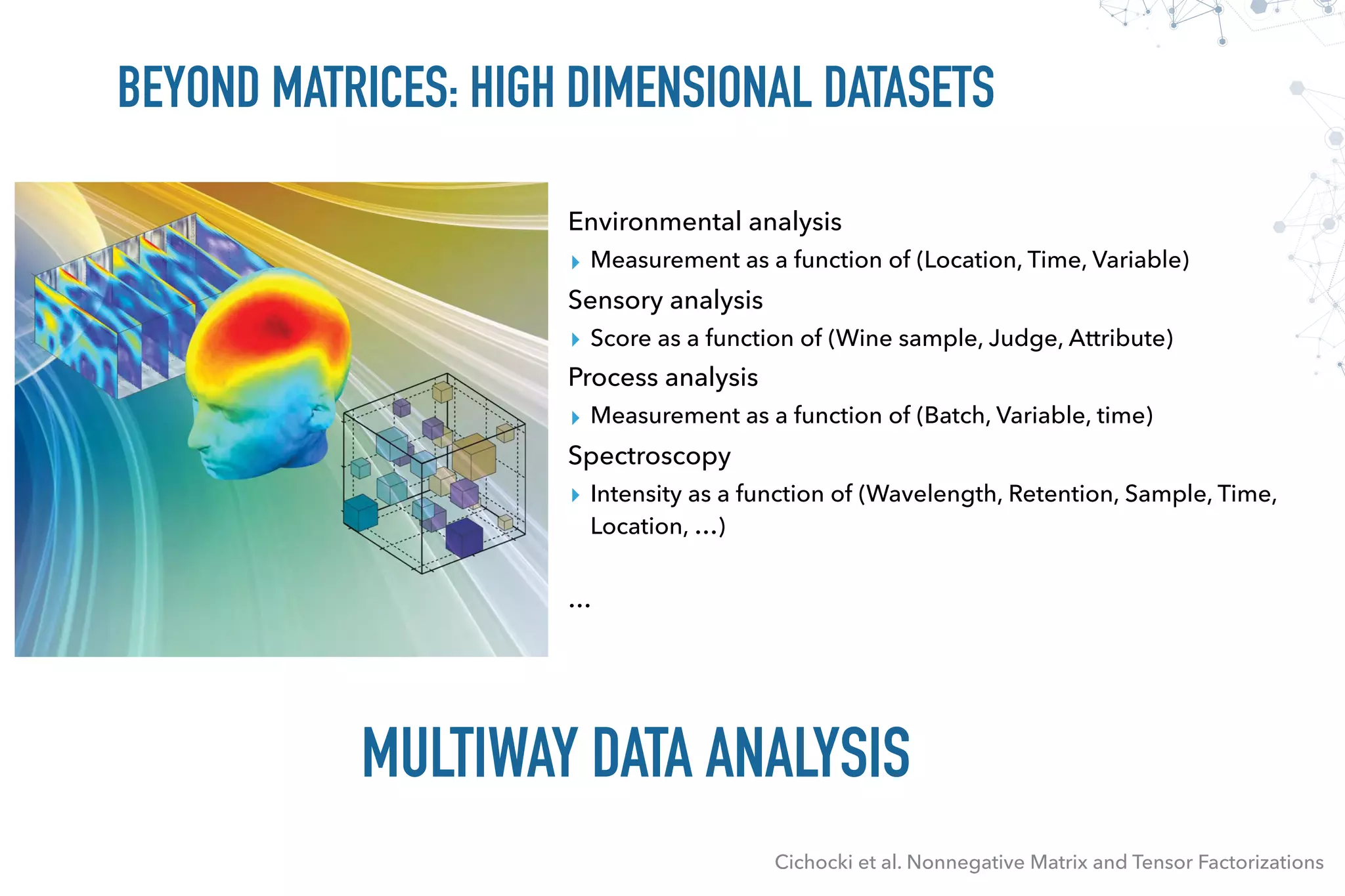


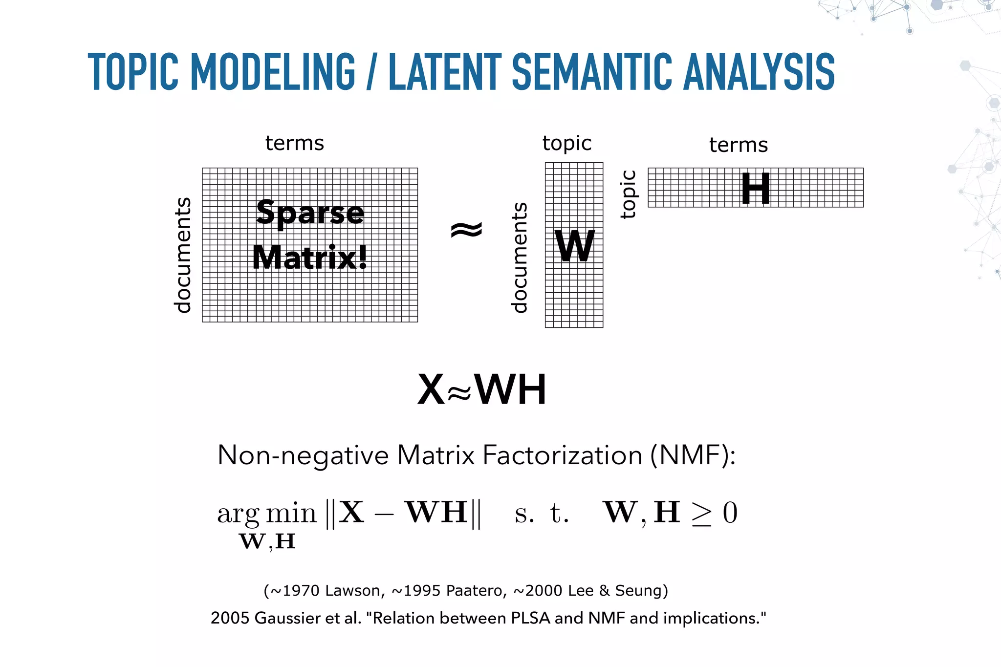
![FIBERS AND SLICES
Cichocki et al. Nonnegative Matrix and Tensor Factorizations
Column (Mode-1) Fibers Row (Mode-2) Fibers Tube (Mode-3) Fibers
Horizontal Slices Lateral Slices Frontal Slices
A[:, 4, 1] A[1, :, 4] A[1, 3, :]
A[1, :, :] A[:, :, 1]A[:, 1, :]](https://image.slidesharecdn.com/pycon8-firenze-170409104152/75/TENSOR-DECOMPOSITION-WITH-PYTHON-18-2048.jpg)
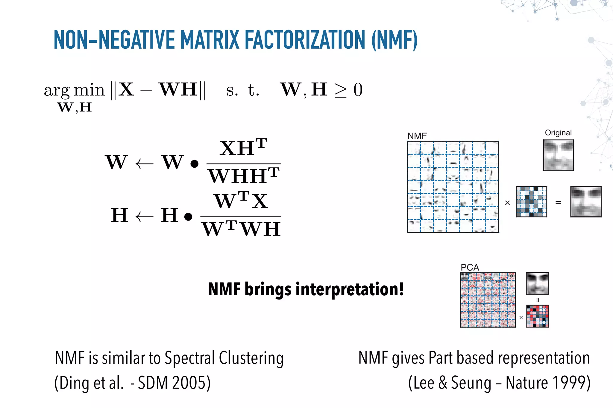
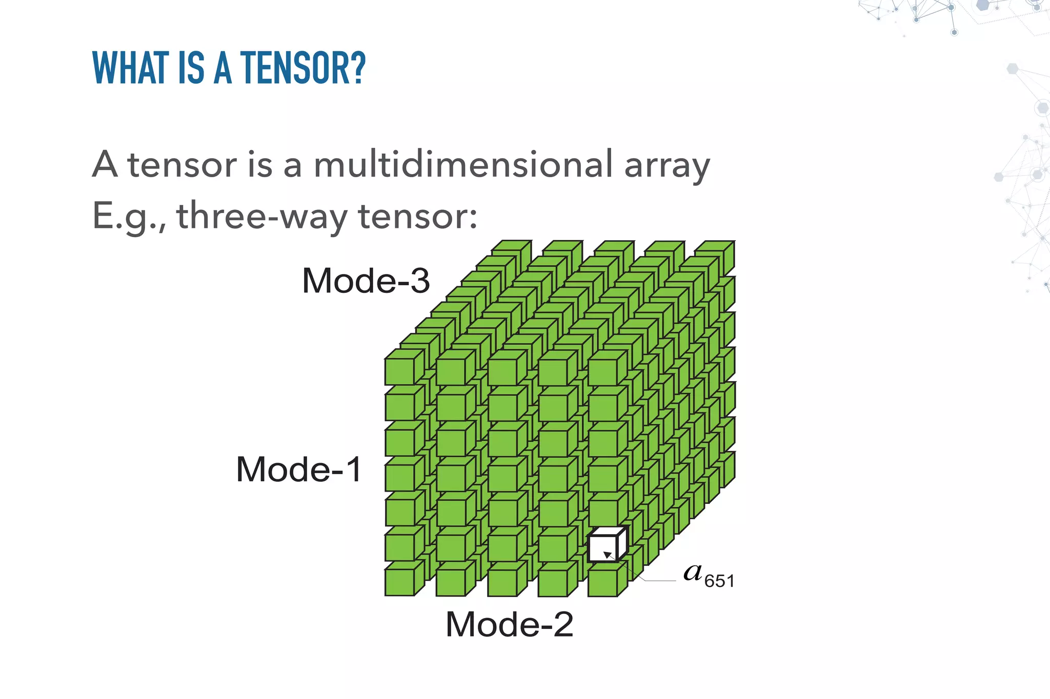
![>>> T = np.arange(0, 24).reshape((3, 4, 2))
>>> T
array([[[ 0, 1],
[ 2, 3],
[ 4, 5],
[ 6, 7]],
[[ 8, 9],
[10, 11],
[12, 13],
[14, 15]],
[[16, 17],
[18, 19],
[20, 21],
[22, 23]]])
OK for dense tensors: use a combination
of transpose() and reshape()
Not simple for sparse datasets (e.g.: <authors, terms, time>)
for j in range(T.shape[1]):
for i in range(T.shape[2]):
print T[:, i, j]
[ 0 8 16]
[ 2 10 18]
[ 4 12 20]
[ 6 14 22]
[ 1 9 17]
[ 3 11 19]
[ 5 13 21]
[ 7 15 23]
# supposing the existence of unfold
>>> T.unfold(0)
array([[ 0, 2, 4, 6, 1, 3, 5, 7],
[ 8, 10, 12, 14, 9, 11, 13, 15],
[16, 18, 20, 22, 17, 19, 21, 23]])
>>> T.unfold(1)
array([[ 0, 8, 16, 1, 9, 17],
[ 2, 10, 18, 3, 11, 19],
[ 4, 12, 20, 5, 13, 21],
[ 6, 14, 22, 7, 15, 23]])
>>> T.unfold(2)
array([[ 0, 8, 16, 2, 10, 18, 4, 12, 20, 6, 14, 22],
[ 1, 9, 17, 3, 11, 19, 5, 13, 21, 7, 15, 23]])](https://image.slidesharecdn.com/pycon8-firenze-170409104152/75/TENSOR-DECOMPOSITION-WITH-PYTHON-20-2048.jpg)
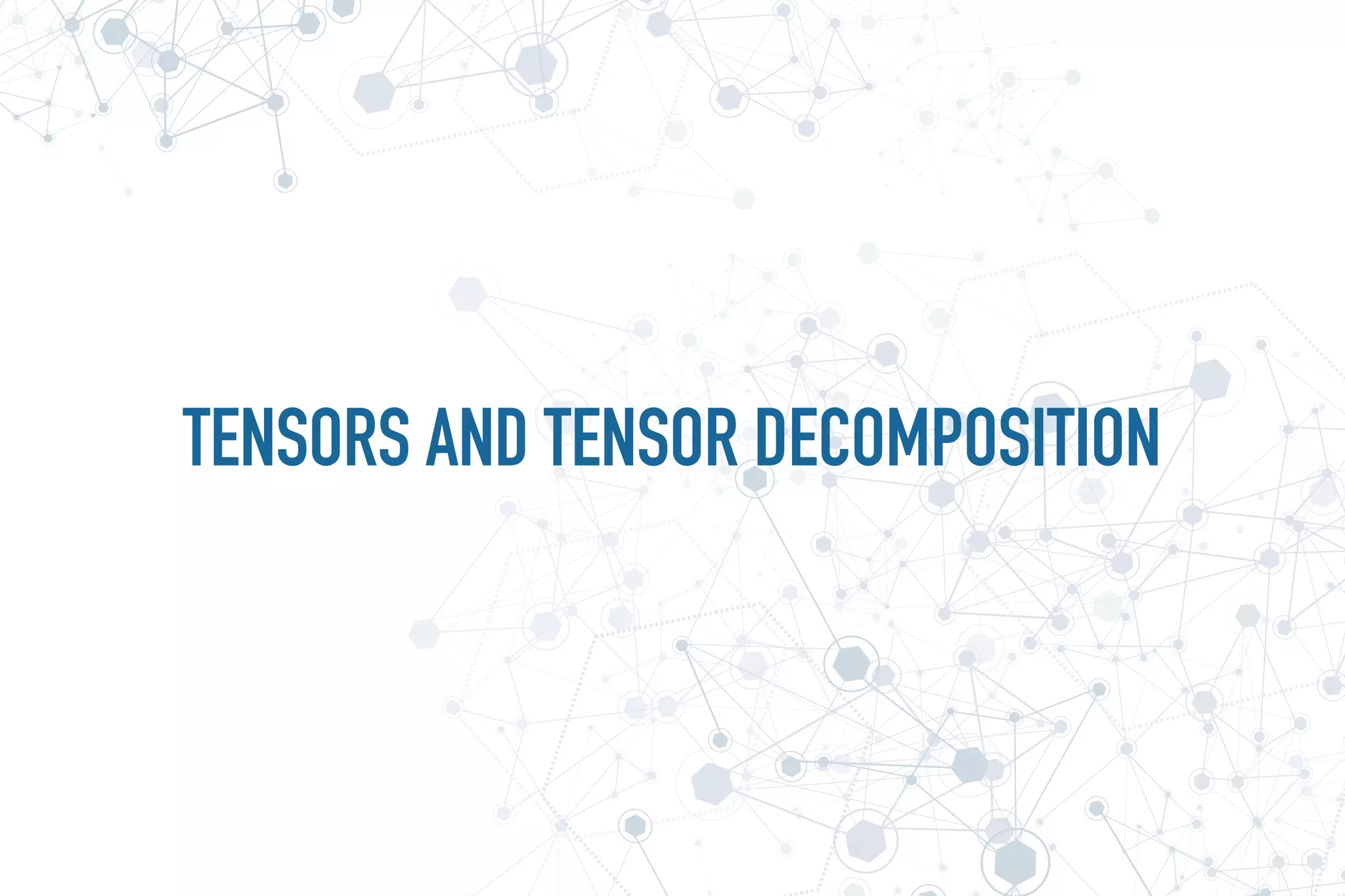
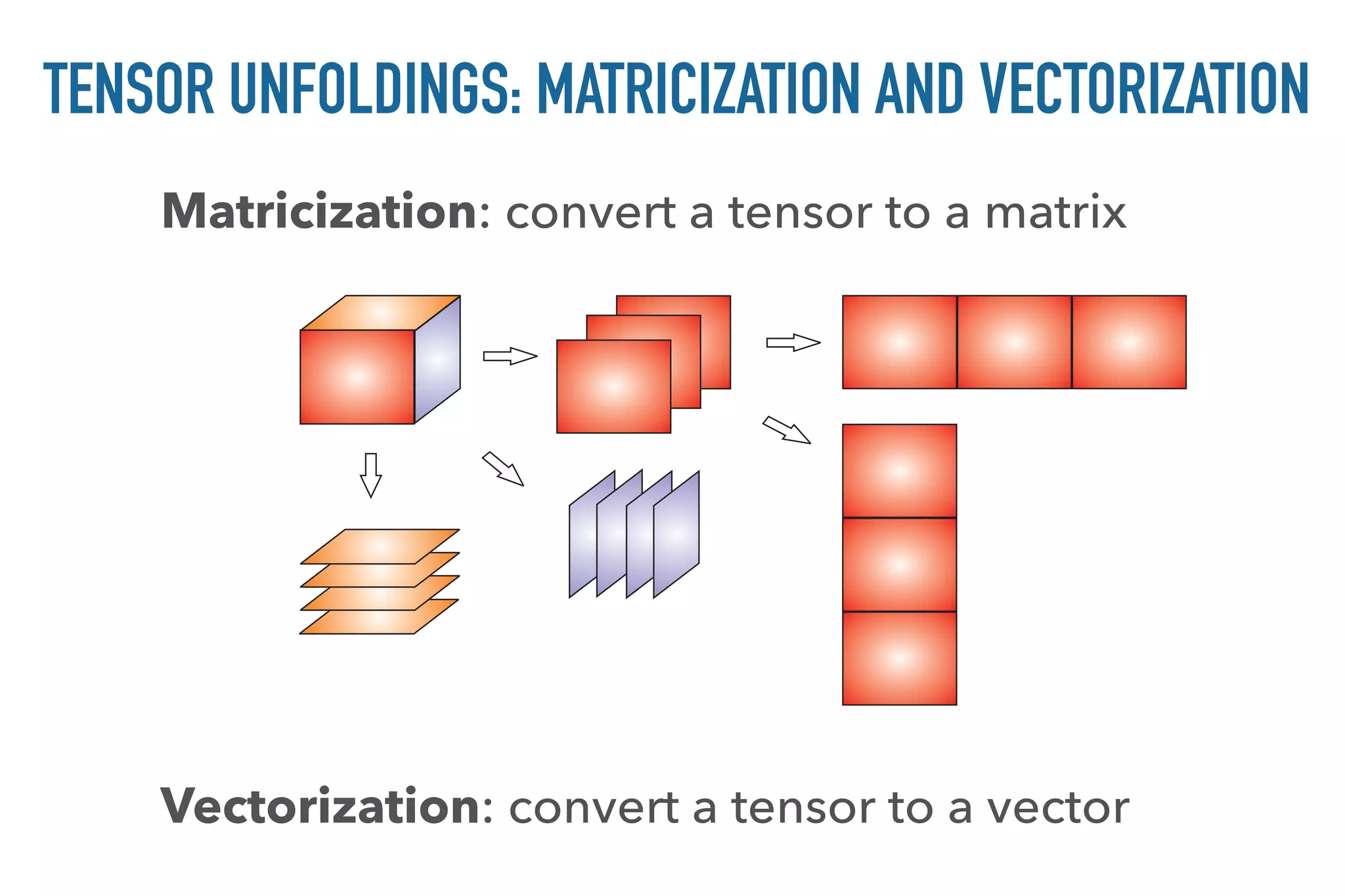
![RANK-1 TENSOR
The outer product of N vectors results in a rank-1 tensor
array([[[ 1., 2.],
[ 2., 4.],
[ 3., 6.],
[ 4., 8.]],
[[ 2., 4.],
[ 4., 8.],
[ 6., 12.],
[ 8., 16.]],
[[ 3., 6.],
[ 6., 12.],
[ 9., 18.],
[ 12., 24.]]])
a = np.array([1, 2, 3])
b = np.array([1, 2, 3, 4])
c = np.array([1, 2])
T = np.zeros((a.shape[0], b.shape[0], c.shape[0]))
for i in range(a.shape[0]):
for j in range(b.shape[0]):
for k in range(c.shape[0]):
T[i, j, k] = a[i] * b[j] * c[k]
T = a(1)
· · · a(N)
=
a
c
b
Ti,j,k = a
(1)
i a
(2)
j a
(3)
k](https://image.slidesharecdn.com/pycon8-firenze-170409104152/75/TENSOR-DECOMPOSITION-WITH-PYTHON-21-2048.jpg)
![array([[[ 61., 82.],
[ 74., 100.],
[ 87., 118.],
[ 100., 136.]],
[[ 77., 104.],
[ 94., 128.],
[ 111., 152.],
[ 128., 176.]],
[[ 93., 126.],
[ 114., 156.],
[ 135., 186.],
[ 156., 216.]]])
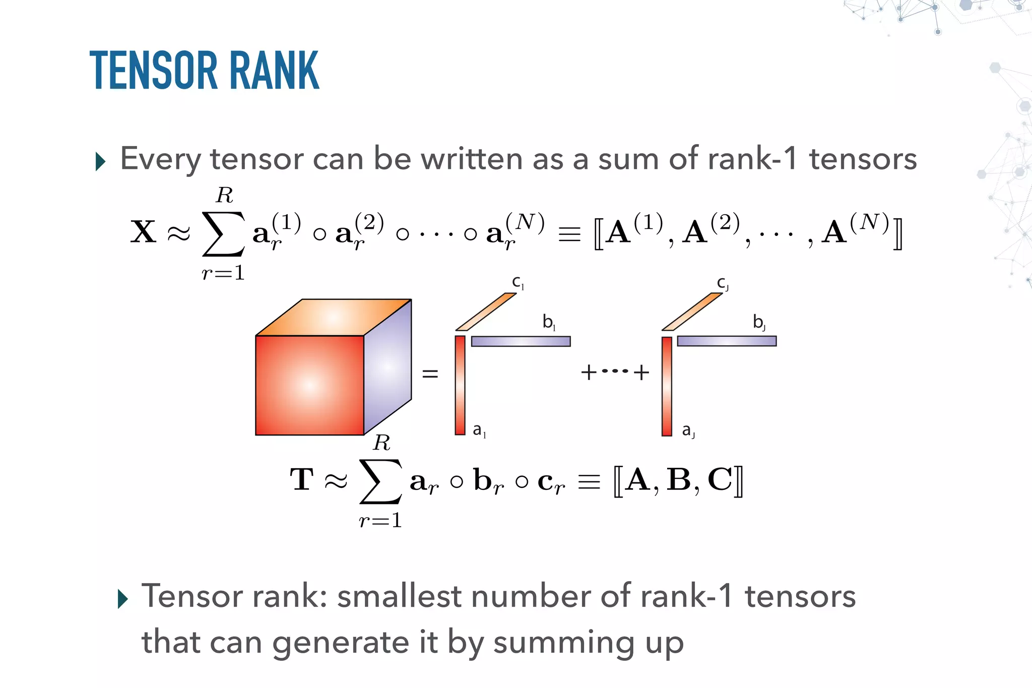
A = np.array([[1, 2, 3],
[4, 5, 6]]).T
B = np.array([[1, 2, 3, 4],
[5, 6, 7, 8]]).T
C = np.array([[1, 2],
[3, 4]]).T
T = np.zeros((A.shape[0], B.shape[0], C.shape[0]))
for i in range(A.shape[0]):
for j in range(B.shape[0]):
for k in range(C.shape[0]):
for r in range(A.shape[1]):
T[i, j, k] += A[i, r] * B[j, r] * C[k, r]
T = np.einsum('ir,jr,kr->ijk', A, B, C)
: Kruskal Tensorbr cr ⌘ JA, B, CK](https://image.slidesharecdn.com/pycon8-firenze-170409104152/75/TENSOR-DECOMPOSITION-WITH-PYTHON-23-2048.jpg)
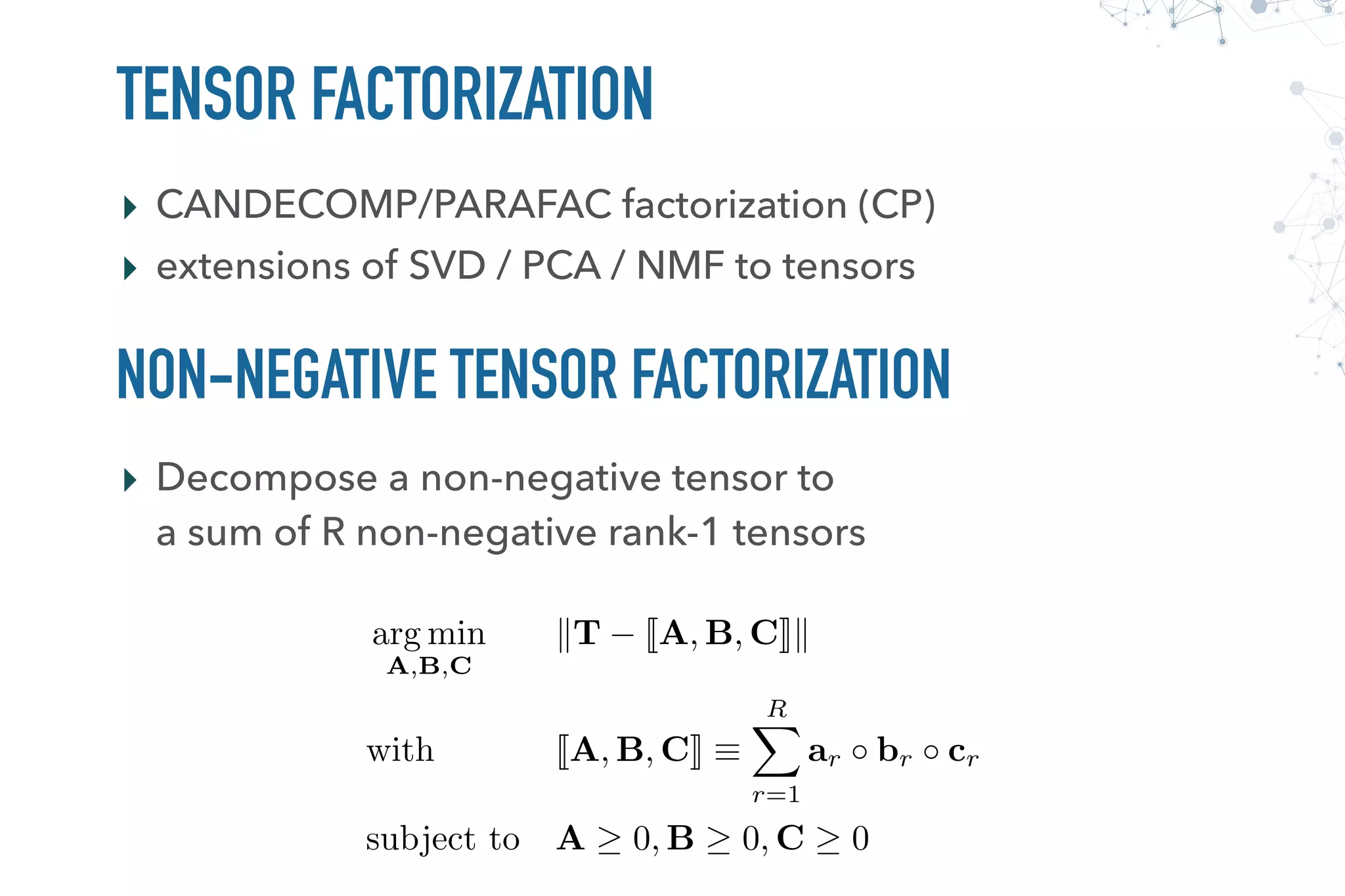
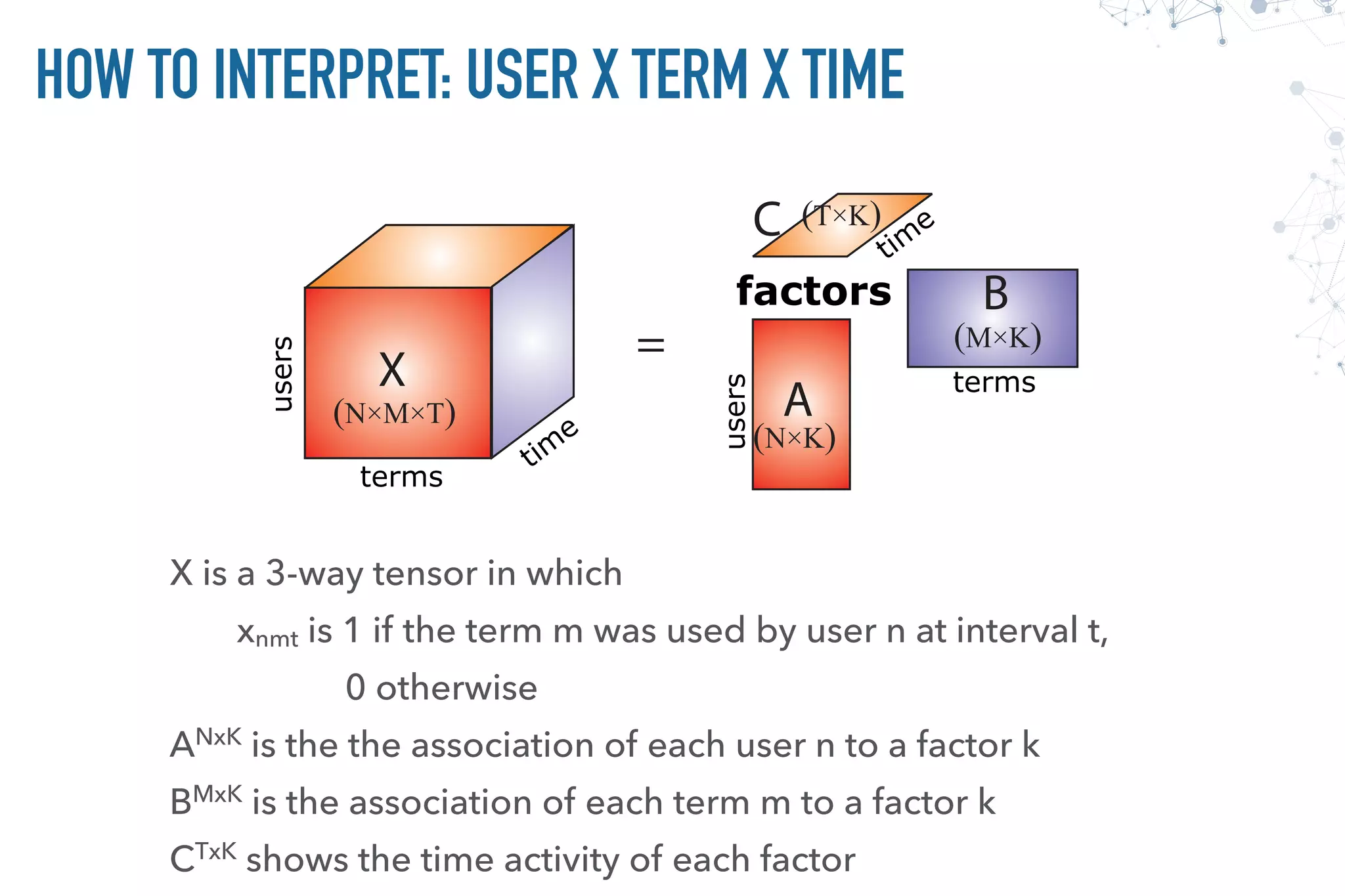
![TENSOR FACTORIZATION: HOW TO
Alternating Least Squares(ALS):
Fix all but one factor matrix to which LS is applied
min
A 0
kT(1) A(C B)T
k
min
B 0
kT(2) B(C A)T
k
min
C 0
kT(3) C(B A)T
k
denotes the Khatri-Rao product, which is a
column-wise Kronecker product, i.e., C B = [c1 ⌦ b1, c2 ⌦ b2, . . . , cr ⌦ br]
T(1) = ˆA(ˆC ˆB)T
T(2) = ˆB(ˆC ˆA)T
T(3) = ˆC(ˆB ˆA)T
Unfolded Tensor
on the kth mode](https://image.slidesharecdn.com/pycon8-firenze-170409104152/75/TENSOR-DECOMPOSITION-WITH-PYTHON-25-2048.jpg)
![F = [zeros(n, r), zeros(m, r), zeros(o, r)]
FF_init = np.rand((len(F), r, r))
def iter_solver(T, F, FF_init):
# Update each factor
for k in range(len(F)):
# Compute the inner-product matrix
FF = ones((r, r))
for i in range(k) + range(k+1, len(F)):
FF = FF * FF_init[i]
# unfolded tensor times Khatri-Rao product
XF = T.uttkrp(F, k)
F[k] = F[k]*XF/(F[k].dot(FF))
# F[k] = nnls(FF, XF.T).T
FF_init[k] = (F[k].T.dot(F[k]))
return F, FF_init
min
A 0
kT(1) A(C B)T
k
min
B 0
kT(2) B(C A)T
k
min
C 0
kT(3) C(B A)T
k
arg min
W,H
kX WHk s.
J. Kim and H. Park. Fast Nonnegative Tensor Factorization with an Active-set-like Method.
In High-Performance Scientific Computing: Algorithms and Applications, Springer, 2012, pp. 311-326.
W W •
XHT
WHHT
T(1)(C B)](https://image.slidesharecdn.com/pycon8-firenze-170409104152/75/TENSOR-DECOMPOSITION-WITH-PYTHON-26-2048.jpg)


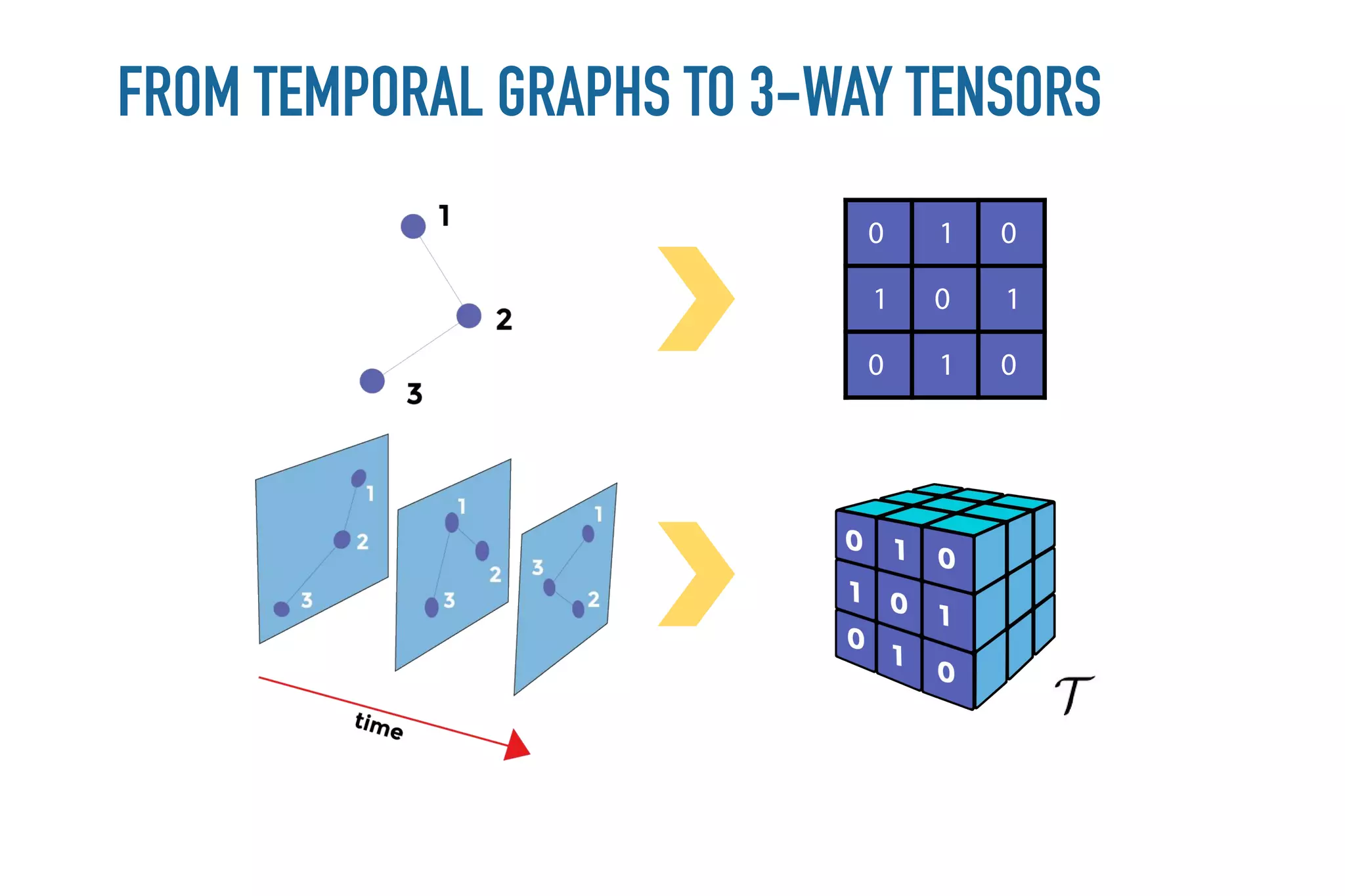
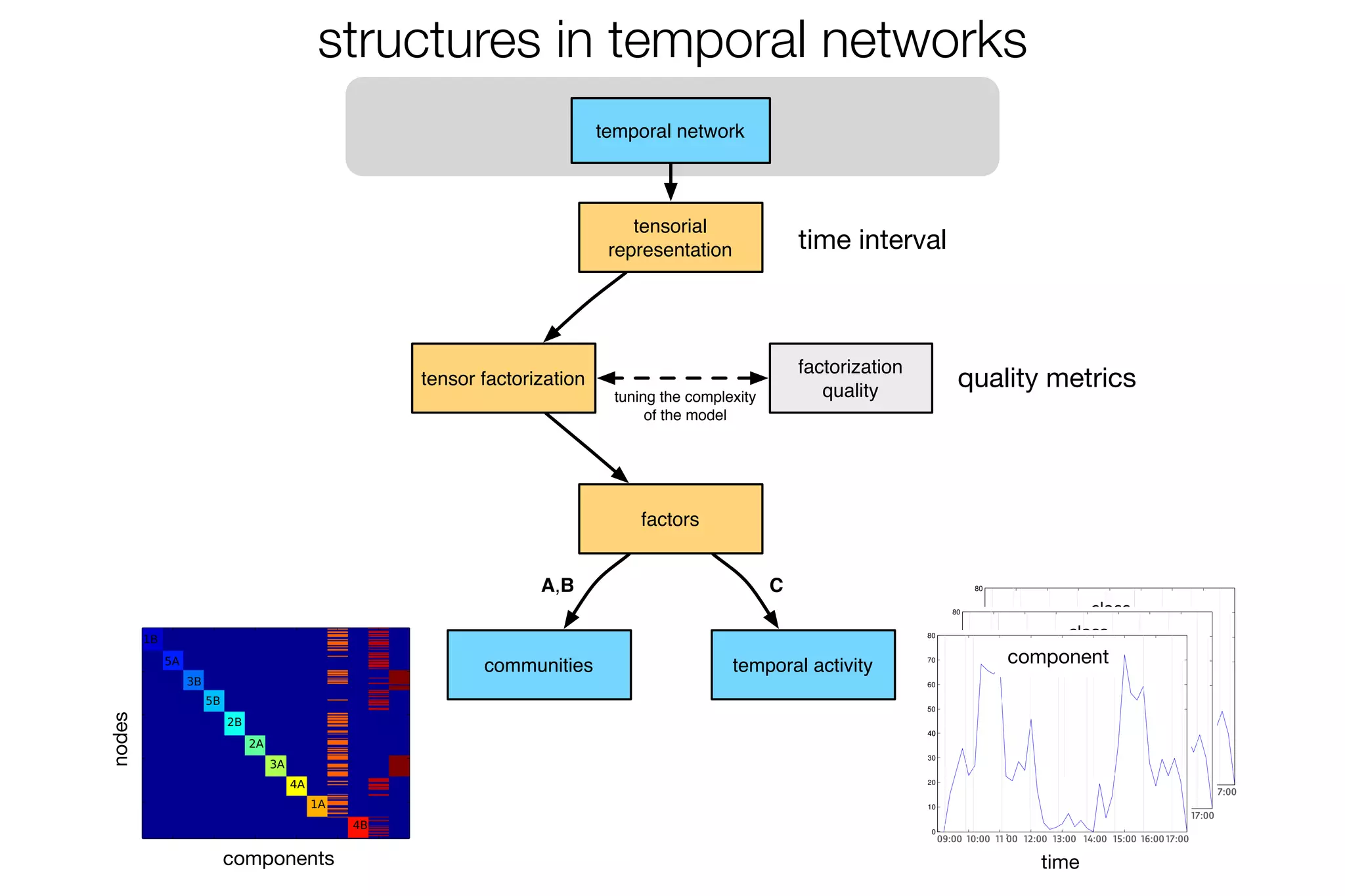


This document discusses tensor decomposition with Python. It begins by explaining what tensor decomposition and factorization are, and how they can be used to represent multi-dimensional datasets and perform dimensionality reduction. It then discusses matrix and tensor factorization methods like NMF, topic modeling, and CP/PARAFAC decomposition. The remainder of the document provides examples of tensor decomposition using Python tools and libraries, and discusses applications to analyzing temporal network and sensor data.


![[Ridge-i 論文読み会] ICLR2019における不完全ラベル学習](https://cdn.slidesharecdn.com/ss_thumbnails/yomikaiiclr2019-190510070433-thumbnail.jpg?width=640&height=640&fit=bounds)