1) The document provides a tutorial on using formulas in Excel, including how to enter formulas, use relative and absolute cell references, perform calculations on ranges of cells, and sum columns of data. 2) It includes steps to enter sample data, calculate values like x-squared and frequencies multiplied by x and x-squared, and use formulas to automatically calculate those values down a column. 3) The tutorial concludes with instructions to sum the sample data columns, enter the student's name, save the Excel file, and provide a printout.

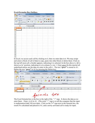
1. Excel-Formulas Box Outlines
In Excel, we access each cell by clicking on it, then we enter data in it. We may swipe
and select a block of cell of data to copy, paste into other block or delete them. Click on
the top left most cell, a border appears, indicating it is selected. In the box above it, A1 is
shown as its’ position, indicating it is in column A, row 1. Enter qwer (In this tutorial all
underlined entries are the data we enter in the cells ). The text “qwer” is stored in A1.
Delete the text “qwer” in A1 by pressing the Delete-key.
The Excel formula-box is the box to the right of the “=” sign. It shows the data as we
enter them . Enter =1+2 in A1. (The extra “=” sign is to tell the computer that the input
is mathematical data, not text data). Click on the “=” sign next to the formula box, the
result 3 is calculated and placed in A1, and a newly activated cell is ready for input.

2. Enter the following data starting from A1 for x, to 0 for z in C4:
x y z
1 2 5 These data are stored from A1 to C4. (We write A1: C4 if we want to
2 4 7 access this block of data. Hence A2: C2 will be the entries 1, 2, 5)
3 6 0 A2:C4 is the corresponding 3x3 matrix.). Click-select D2, enter the data
=A2+B2+C2 , press “Enter”, the sum 8 of the 2nd rows is stored in D2.
Now, we will extend this row sum to the 3rd and 4th rows. Click on D2 and place the
curser at the lower right corner so the curser turns from the larger open cross into a
smaller solid cross, drag this solid cross downward to cover D3, and D4, then release the
mouse. The sum-calculation of the 2nd row is carried to the 3rd and 4th rows, and we get
the sums of 13 and 9 in D3 and D4 respectively. This is called relative referencing, that
is, Excel calculated the result using the cells in the corresponding (relative) positions
used in the computation D2. Hence we have automatically A3+B3+C3 in D3, and
A4+B4+C4 in D4.

3. The syntax for the formula-box is the standard mathematics syntax. Taking power is
written using the ^ symbol, hence x2 is entered as x^2.
In the following tutorial, we will enter data x and sort the data, enter frequencies f’s, find
x2, find f*x, and f*x2 and calculate their sums. These are the calculations needed for
variance and standard deviation.
Open a new Excel sheet. Enter the headers x in A1, f in B1, x^2 in C1, f*x in D1,
f*x^2 E1.
(Entering and sorting data): Enter the data 4, 2, 3, 3 in A2 to A5. Place the open-cross in
A
A2, drag it to A5 and release to shade select the data from A2 to A5. Click the Z↓icon
on the menu bar. This sorts the data in the ascending order. Enter the following
frequencies 5, 2, 1, 3 from B2 to B5.
(Using formula and passing calculation): Place the curser in C2, enter =A2^2 and click
on the “=” next to the formula box, Excel returns the value 4 for 22. Pass this calculation
down column B by placing the curser at the lower right corner of C2 and drag it to C5
and release the button. We obtain the values for the x2, 4, 9, 9, 16 in column C.
Place the curser in D2, enter =A2*B2 and click on the “=” next to the formula box,
Excel returns the value 10 for 5*2. Pass this calculation down column D by placing the
curser at the lower right corner of D2 and drag it to D5 and release the button. We obtain
the values for the f*x.
Place the curser in E2, enter =B2*C2 and click on the “=” next to the formula box,
Excel returns the value 5*22=20. Pass this calculation down column E by placing the
curser at the lower right corner of E2 and drag it to E5 and release the button. We obtain
the values for the f*x2.
(Summing) To sum column A, place the curser in A2 and drag it to A6 to select A2 to
A6, then click on the Σ symbol in the menu bar. The sum of A2 to A5 in stored in A6.
To sum multiple columns, place the curser in B2 and drag it to E6 to select the block
B2 to A6, then click on the Σ symbol in the menu bar. The sum of each column is in
stored in sixth cell.
Finally, in cell A5 enter you name.
Excel files are saved with the extension .xls. Make a print out. Hand it on 4/16.
(End of the tutorial)
FM SU/2011