Full download : https://goo.gl/1JY9aa Introduction to Engineering Experimentation 3rd Edition by Wheeler Solutions Manual

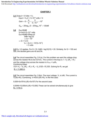
1. 3.1
CHAPTER 3
3.1 Output = 5 Volts = Vo
Input = 5 V = 510-6 volts = Vi
Gain G
V
V
G G dB
o
i
dB
  


  

5
5 10
10
20 20 10 120
6
6
10 10
6
log log
3.2 GdB=60dB
Vi=3mV=310-3 volts
GdB=60dB=20log10G
3dB= log10G
 G = 103
 G = Vo/Vi
Vo = GVi = 103(310-3)
= 3 volts
3.3 Eq. 3.2 applies. For G =10, GdB = log10(10) = 20. Similarly, for G = 100 and
500, the decibel gains are 40 and 54.
3.4 The circuit resembles Fig. 3.9 (a). For this problem we want the voltage drop
across the resistor Rs to be 0.01xVs. The current in the loop is )/( iss RRVI 
and the voltage drop across the resistor is Vdrop = IsxRs.
Combining these:
120)120/()/(01.0 ississs RVRRRVV  . Solving for Ri, we get
Ri = 11,880 .
3.5 The circuit resembles Fig. 3.9(a). The input voltage, Vi, is IxRi. The current is
Vs/(Rs+Ri). Combining, Vi=RixVs/(Rs+Ri). In the first case:
0.005=5x106xVs/(Rs+5x106) For the second case:
0.0048=10,000xVs/(Rs+10,000) These can be solved simultaneously to give
Rs = 416 .
Introduction To Engineering Experimentation 3rd Edition Wheeler Solutions Manual
Full Download: http://testbankreal.com/download/introduction-to-engineering-experimentation-3rd-edition-wheeler-solutions-man
This is sample only, Download all chapters at: testbankreal.com

2. 3.2
3.6 a) From Eq. 3.14,
G
R
R
R
R
R
R
 
 

1
100 1
99
2
1
2
1
2
1
Since R1 and R2 typically range from 1k to 1M, we arbitrarily choose:
R2=99k
 R1 = 1k
b) f = 10 kHz = 104 Hz
GPB = 106 Hz for 741
G = 100
From Eq. 3.15,
f
GPB
G
Hz
Hzc   
10
100
10
6
4
This is the corner frequency so signal is -3dB from dc gain.
dc gain = 100 = 40dB. Gain at 104 Hz is then 37 dB.
From Eq. 3.16,


 





  





     
tan tan1 1
4
4
10
10 4
45
f
fc
o

3. 3.3
3.7
G
R
R
R
R
R
R
 
 

1
100 1
99
2
1
2
1
2
1
Selecting R1 = 1k, R2 can be evaluated as 99k..
Since GBP = 1 MHz = 100(Bandwidth)
 bandwidth = 10 kHz = fc
Gain will decrease 6dB from DC value for each octave above 10 kHz.
The phase angle can be determined from Eq. 3.16,
  







tan 1 f
fc
f(Hz) 0 5k 10k 100k
 0 -26.6 -45 -84.3

4. 3.4
3.8
G
R
R
R
R
  

1000 1
999
2
1
2
1
Selecting R2 = 999 k, R1 can be evaluated as 1 k.
Since GBP = 1MHz for the A741C op-amp and G = 1000 at low
frequencies,
GBP = 1MHz = 1000(Bandwidth)
 Bandwidth = 1 kHz = fc
If f = 10 kHz and fc = 1 kHz, we must calculate the number of times fc
doubles before reaching f.
f f
x
c
x
x
 
 
 
2
1000 2 10000
332.
Now the gain can be calculated knowing that for each doubling the gain
decreases by 6dB (i.e. per octave)
Gain dB dB
dB
( ) log . ( ) 

20 1000 332 6
40
10
From Eq. 3.16,
  







tan 1 f
fc
 






 

tan
.
1 10000
1000
84 3o

5. 3.5
3.9 G = 100 (Actually -100 since signal inverted)
Input impedance = 1000  R1
From Eq. 3.17,
G
R
R
R
R k
 
 
 
2
1
2
2
100
1000
100 
Since GPBnoninv = 106 Hz, from Eq. 3.18,
 
GPB
R
R R
GPB
Hz
inv noninv



 
2
1 2
6
5
100000
1000 100000
10
9 9 10.
From Eq. 3.15,
f
GPB
G
kHzc  


9 9 10
100
9 9
5
.
.
3.10 G = 10 (Actually -10 since output inverted)
Input impedance = 10 k = 10000   R1
From Eq. 3.17,
G
R
R
R
R k
 
 
 
2
1
2
2
10
10000
100 
Since GPBnoninv = 106Hz, from Eq. 3.18,
 
GPB
R
R R
GPB
kHz
inv noninv




2
1 2
6100000
10000 100000
10
909
From Eq. 3.15,
f
GPB
G
kHzc  


0 909 10
10
90 9
3
.
.

6. 3.6
3.11 (a) 10 = 2N. N = ln10/ln2 = 3.33
(b) dB/decade = NxdB/octave = 3.33x6 = 20 dB/decade
3.12
The gain of the op-amp itself is
Vo=g(Vp  Vn) [A]
Vp is grounded so Vp = 0 [B]
The current through the loop including Vi, R1, R2, and Vo is
I
V
R
V V
R R
L
i o
 



 1 2
Vn can then be evaluated as
 V V I R V
R V V
R R
n i L i
i o
   


1
1
1 2
[C]
Substituting [C] and [B] into [A]
 V g V
R V V
R R
o i
i o
  








1
1 2
Rearranging:
   V R R gR V R R R g
V
V
G
R g
R R gR
o i
o
i
1 2 1 1 2 1
2
1 2 1
     
 

 
Noting the g is very large
G
R
R
  2
1

7. 3.7
3.13 The complete circuit is as follows,
For a loading error of 0.1%, the voltage drop across Rs should be
900.001 = 0.09 V. The current through Rs is then:
I
V
R
AR
R
s
S
s
  
0 09
10
0 009
.
.
IRs also flows through R1 and the combination of R2 and Ri. For R2 and Ri,
we have:
V IR
R R R k
R
o
i
  




























10 0 009
1
1 1
0 009
1
1 1
100
1124
2 2
2
. .

The voltage drop across R1=900.0910= 79.91V
R
V
I
1
79 91
0 009
8879 0  
.
.
. 

8. 3.8
3.14
a) If we ignore the effects of Rs and R0, we can use Eq. 3.19:
V
V
R
R R
R
R
R
o
i




 
2
1 2
2
2
2
8
120 100000
7142 9. 
(If we include Rs and R0 ,the value of
R2 is 7193 , less than 1%
different.)
b) I
V
R
V
R R
As
 




 1 2
120
100000 7142 9
0 00112
.
. (neglecting load
effects)
 P = I2R = (0.0012)2(100000 + 7142.9) = 0.13 W
c)
I
V
R
A
A  
 












 


120
0 5 100000
1
1
7142 9
1
10
120
0 5 100000 7092 2
0 00112
6
.
.
. .
.
Voltage drop across line load resistor
V I R V smallA   0 00112 0 5 0 00056. . . ( )
3.15 If f1 = 7600 Hz and f2 = 2100 Hz then the following equation may be used,
f2  2x = f1 where x = # octaves
Substituting,
2100 2 7600
2 3 619
2 3 619
1856
 


 
x
x
x
x octaves
.
log log .
.
Rs
R1
R2 R0
IA
120V

9. 3.9
3.16 fc = 1kHz = 1000Hz , Butterworth
Rolloff = 24 dB/octave
A V
f kHz Hz
f kHz Hz
out1
1
2
010
3 3000
20 20000

 
 
.
Since Rolloff = 24 dB/octave = 6n dB/octave,
 n = 4
From Eq. 3.20,
 
 
G
f fc
n1
1
2
2 4
1
1
1
1 3000 1000
0 01234






.
A
A
G
V A in1in
1out
1
2
010
0 01234
81   
.
.
.
From Eq. 3.20,
 
G2 2 4
1
1 20000 1000
0 00000625




.
 A G A mVout in2 2 2 0 00000625 81 0 051  . ( . ) .
3.17 Using Eq. 3.2, )6.5/(log202 10 oV . Solving, Vo = 4.45
3.18 We want a low-pass filter with a constant gain up to 10 Hz but a gain of
0.1 at 60 Hz. Using Eq. 3.20:
 
 
G
f fc
n
n




1
1
01
1
1 60 10
1
2
2
.
Solving for n, we get 1.28. Since this is not an integer, we select n = 2. With this
filter, the 10 Hz signal will be attenuated 3 dB. If this is a problem, then a higher
corner frequency and possibly a higher filter order might be selected.

10. 3.10
3.19 We want a low-pass filter with a constant gain up to 100 Hz but an
attenuation at 1000 Hz of 20log10 0.01= -40 dB (G = 0.01). Using Eq. 3.20:
 
 
G
f fc
n
n




1
1
0 01
1
1 1000 100
1
2
2
.
Solving for n, we get n = 2
With the selected corner frequency, the 100 Hz signal will be attenuated 3dB. If
this were to be a problem, a higher corner frequency would be required and also
a higher order filter.
3.20 fc = 1500 Hz
f = 3000 Hz
a) For a fourth-order Butterworth filter
n = 4
From Eq. 3.20,
 
 
G
f f
dB
c
n




 
 

1
1
1
1 3000 1500
0 0624 6 24%
24
2
2 4
. .
b) For a fourth-order Chebeshev filter with 2 dB ripple width
n = 4
Frequency Ratio
f
fc
 
3000
1500
2
From Fig. 3.18 we see that for n = 4 and f/fc = 2,
G(dB) = 34dB
c) For a fourth-order Bessel filter
n = 4
Frequency Ratio
f
fc
 
3000
1500
2
From Fig. 3.20 we see that for n = 4 and f/fc = 2,
G(dB) = 14 dB

11. 3.11
3.21
n
G
f kHz
R
c




1
1
12
10001 
At dc, Eqs. 3.21 and 3.17 are equivalent. Since we require no gain, set R1 = R2.
Thus, R1 = R2 = 1000
From Eq. 3.26, we can calculate C,
f
R C
kHz
C
C F
c 

 
1
2
12
1
2 1000
0 013
2


( )
.
3.22 It would not be possible to solve problem 3.16 using a simple Butterworth
filter based on the inverting amplifier. This is because R1 would have to be on the
order 10 M. Such a resistance is higher than resistances normally used for
such circuits because it is on the order of various capacitive impedances
associated with the circuit. The signal should first be input to an amplifier with a
very high input impedance such as a non-inverting amplifier and the signal then
passed through a filter.
3.23
n
G
f Hz
f kHz
c




4
1
1500
25
From Eq. 3.20,
 
 
G
f fc
n




 


1
1
1
1 25000 1500
130 10
2
2 4
5
.
GdB = 20log10(1.310-5)
3.24 VdivVDeflectionVin 6.823.4/ 

12. 3.12
3.25 mVmVdivVDeflectionMaximumRange 8001008/ 
3.26 The visual resolution is on the order of the beam thickness (for thick beams
is may be on the order of ½ the beam thickness since one can interpolate within
the beam. Taking the resolution as the beam thickness, the fractional error in
reading is 0.05/1 = 0.05 (5%). In volts the resolution is 0.05x5 mV = 0.25 mV.
3.21
n
G
f kHz
R
c




1
1
12
10001 
At dc, Eqs. 3.21 and 3.17 are equivalent. Since we require no gain, set R1 = R2.
Thus, R1 = R2 = 1000
From Eq. 3.26, we can calculate C,
f
R C
kHz
C
C F
c 

 
1
2
12
1
2 1000
0 013
2


( )
.
3.22 It would not be possible to solve problem 3.16 using a simple Butterworth
filter based on the inverting amplifier. This is because R1 would have to be on the
order 10 M. Such a resistance is higher than resistances normally used for
such circuits because it is on the order of various capacitive impedances
associated with the circuit. The signal should first be input to an amplifier with a
very high input impedance such as a non-inverting amplifier and the signal then
passed through a filter.

13. 3.13
3.23
n
G
f Hz
f kHz
c




4
1
1500
25
From Eq. 3.20,
 
 
G
f fc
n




 


1
1
1
1 25000 1500
130 10
2
2 4
5
.
GdB = 20log10(1.310-5)
= 97.7 dB
Introduction To Engineering Experimentation 3rd Edition Wheeler Solutions Manual
Full Download: http://testbankreal.com/download/introduction-to-engineering-experimentation-3rd-edition-wheeler-solutions-man
This is sample only, Download all chapters at: testbankreal.com