SlideShare a Scribd company logo
1 of 31
Download to read offline
Hiring uncertainty: a new labour market indicator∗
Ekkehard Ernst†

Christian Viegelahn‡

7 February 2014

Abstract This paper develops a forward-looking indicator for macroeconomic uncertainty that
employers are confronted with when they take decisions about the size of their workforce. The
model that provides the basis for this uncertainty indicator interprets hires and lay-offs of workers
as an investment into projects with uncertain return. Employers decide when to undertake this
investment. Uncertainty can then be derived as a function of a labour productivity threshold
above which it is profitable for employers to hire workers. The measure that is first theoretically
derived is then taken to the data. Economy-wide uncertainty for G7 economies and uncertainty by
economic sector for the United States are calculated from data on hiring demand and unit labour
costs. The resulting quarterly time series demonstrate that in most economies hiring uncertainty
went up at the onset of the Great Recession and has remained at an elevated level since then. A
panel VAR analysis reveals that hiring uncertainty excercises a significant, economically sizeable
and persistent effect on both the output gap and unemployment.

Keywords: Crisis, Employer, Hiring, Risk, Uncertainty, Unemployment

JEL classification: D80, E66, J23, J63

∗ The authors would like to thank Giacomo De Giorgi, Maia G¨ ell and Robert Shimer for comments and sugu
gestions. Any views and opinions expressed in this paper are those of the authors and not necessarily those of the
institutions they are affiliated with.
† Contact address: International Labour Office, Research Department, 4 Route des Morillons, 1211 Geneva,
Switzerland. Email: ernste@ilo.org. Phone: +41 22 799 7791.
‡ Contact address: International Labour Office, Research Department, 4 Route des Morillons, 1211 Geneva,
Switzerland. Email: viegelahn@ilo.org. Phone: +41 22 799 7264.

1
1

Introduction

Five years after the onset of the Great Recession, many labour markets worldwide are stagnant and
high unemployment continues to persist.1 Particularly in advanced economies, hiring activity of
the private sector is still down compared to pre-crisis levels. In the United States, for example, the
number of hires in the private sector as percentage of total employment has decreased significantly
during the crisis. The hiring rate stood at above 4.0 per cent in every month between April 2003
and February 2008, but has consistently been below 4.0 per cent ever since then. According to the
latest data from the US Bureau of Labor Statistics, the hiring rate stood at 3.7 per cent in October
2013, which is still below the hiring rates observed before the crisis. Morissette et al. (2013) find
similar evidence on hiring rates for Canada. Also estimates on unemployment ouflow rates from
the International Labour Office ILO (2013b) point to less hiring activity than before the crisis in
many economies.
Hiring can be seen as a real investment option. When hiring new staff, firms invest into an increase
of their workforce. They incur a sunk cost which includes the costs of recruitment, training and
committed salary payments. In return, they expect that the newly hired workers contribute to
larger profits through their productivity. However, apriori it is uncertain how productive new staff
can be, given that the macroeconomic environment in which workers operate is uncertain. Even
if a firm is perfectly able to assess the skill level of new entrants through appropriate screening
measures in the recruitment process, there is some uncertainty about the return to the investment.
There are external factors beyond the control of an individual firm, in particular economic policy,
that can have an impact on the demand for the firms’ products and services as well as on the
conditions of production. These factors, thus, have a bearing on the return that is generated by
new staff.
There are two potential explanations for meager hiring rates. Either the expected returns from
hiring are too low, so that firms do not expect to generate additional profits by hiring new staff. In
other words, there are no profitable investment projects available to firms. Or the uncertainty about
future returns is too high. So even if there are investment projects available that yield an expected
positive return, it is not certain whether such a return will eventually materialize. As a consequence,
firms may find it optimal to postpone their hiring decision and wait for new information to come
in rather than hiring new workers right away. Several international organizations diagnosed that
1 As the ILO (2013a) reports in its Global Employment Trends 2013 report, the global number of unemployed
is still by 28 million higher than it was before the crisis. For advanced economies this gap amounts to 14 million.

2
uncertainty is likely one of the key factors behind the jobless recovery from the economic crisis that
has been observed in many countries. As the ILO (2013a) argues in its Global Employment Trends
2013 report, the lack of policy coordination and the indecision of policy makers in several countries
has led to uncertainty about future conditions and reinforced corporate tendencies to increase cash
holdings or pay dividends rather than expand capacity and hire new workers. In a similar vein, the
International Monetary Fund stated in 2012 that there is a level of uncertainty which is hampering
decision makers from investing and from creating jobs.2
Uncertainty cannot be directly observed, but needs to be indirectly inferred from decisions that are
influenced by uncertainty. Moreover, there are different types and perceptions of uncertainty. Even
though, measuring uncertainty is hence not straight-forward, the literature has come up with some
methodologies. Baker et al. (2013) developed an economic policy uncertainty index for some of the
largest economies. One component of the index measures the coverage of uncertainty in newspapers
and counts articles that contain certain word combinations relating to economic policy uncertainty.
Another component calculates a measure of forecasters’ disagreement about future prospects of
the economy.3 Bloom et al. (2012) use micro-level data on manufacturing plants and take the
cross-sectional dispersion of productivity shocks as measure for uncertainty. Baum et al. (2006)
estimate conditional variances of industrial production, output, inflation and stock price returns
with GARCH models and interpret them as indicators for macroeconomic uncertainty. Haddow
et al. (2013) combine several indicators of uncertainty such as option-implied volatility of equity
prices and the above-mentioned economic policy uncertainty index into a summary uncertainty
index through principal component analysis.
This paper contributes to this fast-growing literature by proposing a new indicator for macroeconomic uncertainty, measuring the uncertainty that employers face when taking hiring decisions.
For firms as employers, it is particularly uncertainty about future demand and the conditions of
production that can have an impact on their hiring decision. This type of uncertainty, which this
paper refers to as hiring uncertainty, can either arise from sources which can be considered as
beyond direct control of policy makers, such as terrorism or natural desasters. But it can also arise
from uncertainty about economic and financial policies which can directly be influenced by policy
makers through their economic policy decisions or absence thereof.
While existing measures from the literature typically assess uncertainty at an economy-wide level,

2 See

http://www.imf.org/external/pubs/ft/survey/so/2012/surveyartg.htm.
details on the methodology are available at http://www.policyuncertainty.com.

3 More

3
the hiring uncertainty measure that this paper proposes can be derived by economic sector. The
level of uncertainty perceived by employers is very likely to depend on the economic sector in which
these employers are located. The model that underlies the proposed uncertainty measure has its
origin in McDonald and Siegel (1986) who consider the investment decision of a firm.4 This paper
adapts the model to the context of firms’ hiring and lay-off decisions. Firms can decide about
the time when to hire workers or, alternatively, when to lay workers off. They only hire workers
when the expected return to hiring is strictly larger than the sunk costs incurred. The size of
the minimum wedge between return and sunk costs that makes it optimal for firms to invest into
their workforce depends on the degree of uncertainty in the economy. Similarly, firms decide to
lay workers off when their productivity is lower than the costs. In order to derive an empirical
measure on the basis of the theoretical model, this paper introduces the simultaneous investment
decision of all firms in an economy and assumes heterogeneity in productivity across firms. The
level of uncertainty is then calculated in such a way that it is consistent with the hiring and lay-off
plans announced by employers in the economy.
This paper is organized as follows. The next section sets up the theoretical framework on which the
hiring uncertainty indicator introduced in this paper is based on. In order to derive an equation for
uncertainty that can be applied to actual data, section 3 adds firm heterogeneity to this framework
and analyzes the combined decisions of all firms in an economy. Section 4 describes the data that
are used to derive economy-wide hiring uncertainty for G7 economies and hiring uncertainty in
manufacturing and construction for the United States. Section 5 presents and discusses the results.
Section 7 concludes by discussing possible extensions and future work.

2

Theoretical framework

As basis for the hiring uncertainty indicator derived in this paper, this section adapts the model
set up by McDonald and Siegel (1986) to firms’ hiring and lay-off decisions and analyzes when it
is optimal for an individual firm to change the size of its workforce.

4 See

Dixit and Pindyck (1994) for a textbook presentation of the paper.

4
2.1

Hiring decision

Consider a firm i that has the option to hire ai workers which is the exogeneously given number
¯
of workers required to implement a particular project.5 Hiring these workers comes along with a
sunk cost ai Wi with firm-specific labour cost per worker Wi . This sunk cost broadly corresponds
¯
to the wage commitment that is irreversably fixed in the work contracts the firm signs with new
staff.6 The firm expects a return to its investment in the form of the expected value added ai Pit
¯
that is generated by newly hired staff and sold on the market, where Pit denotes firm-specific value
added per worker. For example, assume that there is an advanced notice period of three months
for laying off workers. The wage commitment then corresponds to three months of wage and salary
payments for the newly hired workers. The expected value added is the output that the workers
are expected to produce within these three months.
The expected rate of return on the investment can then be written as Vit =

Pit
Wi ,

where Vit denotes

the expected value added generated by the newly hired workers per unit of sunk cost. Vit will
also be referred to as labour productivity of firm i in quarter t.7 Vit is independent of project size
ai , given that labour costs and productivity are assumed to be the same for all workers hired by
¯
the firm. It is subject to economy-wide productivity shocks and evolves according to a stochastic
process that is described by a geometric Brownian motion as follows:

dVit = ηVit dyt

(1)

where dVit is the change in labour productivity of firm i over the instant from t to t + dt.8 Future
changes in labour productivity are subject to economy-wide productivity shocks that are embedded
into the expression dyt which is a Wiener process, that is, it can be written as
√
dyt =

with

t

t

dt

(2)

as a standard normally distributed random variable with zero mean and a standard devi-

ation of one. Moreover, the random variable

t

is serially uncorrelated so that E[

t s]

= 0 for any

t = s.
5 For example, if the firm hires workers in order to introduce a new product into the market, the firm will hire
the amount of workers that is necessary to produce the optimal quantity that the firm wants to sell on the market.
6 The objective here is to develop an uncertainty measure that can be taken to the data for many countries. As
a consequence, recruitment and training costs for which not much data are available are assumed to be small.
7 This definition of labour productivity is, for example, also found in Altomonte et al. (2012).
8 Only economy-wide productivity shocks are considered, so dy is the same for all firms i.
t

5
The current value of labour productivity is known, so when the firm decides to hire, it knows with
certainty which payoff its decision will yield. In contrast, future labour productivity is uncertain,
so the firm does not know how these payoffs will evolve in the future. Equations (1) and (2) imply
that the future level of labour productivity is distributed log-normally. The variance grows linearly
with the time horizon, so there is less uncertainty about labour productivity tomorrow compared
to one year from now. η provides a measure for the standard deviation of the economy wide shocks.
η will be referred to as hiring uncertainty.
The possibility to hire a worker can be interpreted as an option for the firm to invest in a real
asset. If the firm has the possibility to hire ai workers, it possesses ai Wi units of this option. The
¯
¯
firm optimally chooses time t at which it undertakes the investment and hires workers, assuming
that the time horizon is infinite, so that the solution does not depend on time. The chosen point
of time should maximize the expected net present value of an option which can be written as

F (Vit ) = E [Vit − 1] e−ρt

(3)

where E[...] is the expected value of the project, given information up to time t. ρ is the time
discount factor, which is assumed to be valid economy-wide. The maximization is subject to the
stochastic process for labour productivity that is defined in equation (1).
It can be shown that the solution to this problem consists of a single threshold for productivity
Vih .9 Only if productivity exceeds this value the firm will invest and hire workers. If productivity
is below this threshold, the firm will find it optimal to wait rather than invest into the project.
Since the time horizon is assumed to be infinite, the threshold will not be dependent on time.
To find this threshold, we set up the Bellman equation which describes the value of the option as
the maximum of two possibilities. If the firm invests immediately, it gets Vit − 1. If it instead
waits dt with the investment, it gets the expected continuation value E [F (Vi,t+dt )], discounted
with discount factor ρdt. The Bellman equation can be written as

F (Vit ) = max Vit − 1, E

1
F (Vi,t+dt )
1 + ρ dt

.

(4)

If V < Vih , so that productivity is below the threshold that still needs to be established, then
the second argument of the maximum function exceeds the first one. In other words, the continuation value is larger than the payoff from investing immediately. As a consequence, the following
9 See

Dixit and Pindyck (1994) for technical details.

6
expression holds
1
F (Vi,t+dt ) .
1 + ρ dt

F (Vit ) = E

(5)

which can be transformed by multiplying with (1 + ρ dt) and subtracting F (Vit ) on each side to

ρF (Vit )dt = E [dFit ]

(6)

with dFit = F (Vi,t+dt ) − F (Vit ). Next, we apply Ito’s Lemma and expand dFit as follows:

E [dFit ] =

1 2 2
η Vit F (Vit )dt.
2

(7)

Plugging (7) into (6) and dividing by dt, we obtain the following expression:
1 2 2
η Vit F (Vit ) − ρFit = 0.
2

(8)

This equation needs to be satisfied within the continuation region, when Vit < Vih . But it also
needs to be satisfied at the boundary of the continuation region, when the firm is indifferent
between hiring workers and waiting, so it needs to hold for Vit = Vih .
If Vit > Vih , then the firm will invest and hire workers. In this case, the first argument of the
maximum function in (4) exceeds the second one, so that the payoff from immediately investing is
larger than the continuation value. This implies that

F (Vit ) = Vit − 1.

(9)

This equation holds when Vit > Vih , but it also holds at the boundary, when the firm is indifferent
between hiring workers and waiting. In other words, (9) holds when Vit = Vih which is the socalled value-matching condition. But it is not only that the values of the first and second argument
of the maximum function in (4) should coincide. A further condition is that the first and second
argument of this function have to approach each other tangentially at the threshold value for
h
productivity Vit so that

F (Vit ) = 1

(10)

when evaluated at Vih , the so-called smooth-pasting condition. In order to derive the threshold
productivity value above which it is optimal to invest, we apply the method of undetermined

7
coefficients and guess that the option value can be represented in the form

F (Vit ) = A(Vit )β

(11)

when evaluated at Vih with A and β as constants to be determined. This form of the solution
is the only one that is consistent with the fact that F (0) = 0 which is implied by the stochastic
process defined in equation (1). Once the return to hiring reaches zero, it will stay at zero forever
as well as the option value.
The four conditions (8)-(11) determine the solution for Vih . From substituting (11) into (9) and
(10), the threshold productivity value can be derived as

Vih =

β
.
β−1

(12)

Plugging (9) and (12) into (11), we can solve for A as

A=

(β − 1)β−1
.
ββ

(13)

If we substitute (11) into (8), we obtain
1 2
η β(β − 1) − ρ = 0
2

(14)

which can be solved for β as
β=

1
+
2

1 2ρ
+
> 1,
4 η2

(15)

where only the positive root is considered, given that F (0) = 0. For the threshold productivity
value Vih , equation (15) implies that Vih > 1. In order for the firm to hire workers, it does
not necessarily suffice that a worker generates more value added than it costs. Instead, workers’
productivity has to exceed its cost by a positive amount, given by equation (12). Because of
uncertainty, the return of the project in terms of the net present value of expected future profit
flows has to be strictly larger than the sunk costs in order to make the investment worthwile. This
is the main result of McDonald and Siegel (1986).
Additionally, since ρ and η are economy-wide parameters, we can drop subscript i and write the
productivity threshold for hiring as
Vih = V h .

8

(16)
The productivity threshold above which it is optimal to hire workers is not firm-specific, but valid
for all firms in the economy. Taking (12), (15) and (16) together and solving for uncertainty
parameter η, we can derive
η=

2ρ
h
( V V −1
h

− 1 )2 −
2

1
4

.

(17)

Hiring uncertainty in the economy depends on the discount factor and the productivity threshold,
above which firms hire workers. When taking this equation to quarterly data, we will for each
quarter determine which level of uncertainty is consistent with the data observed in that quarter.
Since hiring uncertainty is constant over time in the model and there is no difference between the
level of current and future uncertainty, the empirical measure that will be derived for each quarter
is forward-looking in nature.

2.2

Lay-off decision

Instead of opening up a new project and hiring, a firm also has the option to scrap an existing
project and lay workers off, where ¯i is the exogeneously given number of workers involved in the
b
project. Laying workers off can be seen as a negative investment. When laying workers off, a
firm obtains the wage commitments ¯i Wi back which can be seen as a return to this investment.
b ¯
However, in exchange it has to relinquish the expected value added ¯i Pit produced by these workers
b
in the future which is an opportunity cost of laying off workers. For example, assume that the
workers would have stayed for one more year working for the firm, but are instead laid off early.
Then the wage commitment “saved” by the firm corresponds to the wages that would have been
paid to the workers within this one year, if they had not been laid off. The expected value added
is the output that these workers would have been expected to produce in the same period.
Let us define again Vit =

Pit
Wi ,

where Vit denotes the expected value added that would have been

generated by the workers that are laid off per unit of labour cost. As for hiring, note that Vit
is independent of project size ¯i , given that labour costs and productivity are assumed to be the
b
same for all workers laid off by the firm. Labour productivity evolves according to the stochastic
process defined in equations (1) and (2).
The lay-off decision problem is solved analoguously to the hiring decision problem. The difference is
that the firm’s return to project scrapping is now

1
Vit ,

the inverse of labour productivity. However,

as for hiring, the possibility to lay off workers can be seen as an option for the firm. The firm aims
at maximizing the expected net present value of this option by choosing the optimal time to lay
9
workers off. The solution consists again of a productivity threshold and the firm will only want to
lay workers off if productivity gets below this threshold, denote by Vil .
The productivity threshold below which firms will lay workers off can be derived as

Vil = V l =

β−1
β

(18)

where β is defined as in equation (15). It should be noted that V l =

1
Vh

. Given the definition

of β, Vih < 1 is now valid. Only when productivity is lower by a strictly positive amount, given
by (18), firms may decide to scrap a project. Hiring uncertainty η can then, as alternative to (17),
also be expressed as
2ρ

η=
1
1−V l

−

1
2

.

2

−

(19)

1
4

Note that this value of η corresponds exactly to the one in (17). The following section will discuss
how equations (17) and (19) are transformed into expressions that can be used to calculate hiring
uncertainty on the basis of available data.

3

Taking theory to the data

In the previous section, hiring uncertainty was derived as a function of the productivity thresholds
V h and V l , where one is the inverse of the other. Since it is not obvious which data can be used
to measure these productivity thresholds, they need to be expressed as functions of variables for
which data are available.
In the economy-wide version of the uncertainty indicator, the productivity thresholds are valid for
the whole economy, assuming that firms in an economy apply the same discount factor and perceive
the same economy-wide uncertainty. In the sectoral version, the productivity thresholds are sectorspecific, assuming that firms in the same sector apply the same discount factor and perceive the
same sectoral uncertainty. Whether a firm hires workers, lays them off or does not change the size
of its workforce depends on where the firm is located in the productivity distribution across firms
in a given moment of time. If a firm’s productivity is below the lower threshold so that Vit ≤ V l ,
then this firm will lay workers off. If it is above the upper threshold so that Vit ≥ V h , the firm
will hire workers. If it is in between the two thresholds so that V l < Vit < V h , the firm will leave
the number of workers in its workforce unchanged.

10
So far, we have not modeled the productivity distribution across firms in a given moment of time.
The previous section has just defined the stochastic process according to which the productivity
of a single firm varies over time with future productivity values being distributed log-normally.
However, in reality the productivity in a given point of time varies across firms. Therefore, we
consider in this section the hiring and lay-off decisions of multiple firms that are heterogeneous in
productivity. On the basis of this extension of the theoretical framework, we can derive the two
productivity thresholds V l and V h that are needed to calculate hiring uncertainty.
In the absence of firm-level data, the productivity distribution across firms in a given moment of
time cannot be observed.10 Nevertheless the exact distribution can be inferred from available data
under certain assumptions. In particular, we will need to assume that productivity is distributed
log-normally across firms. This assumption is in line with the one made in the trade literature
on heterogeneous firms by Melitz (2003) who assumes that firms’ initial productivity is drawn
from a distribution with support (0, inf). There indeed must be a lower threshold of productivity,
given that firms with a productivity below such a threshold are forced to exit the market. The
productivity of these firms hence cannot be observed. Okubo and Tomiura (2013) find that the
productivity of firms located in peripheral regions of Japan is close to log-normally distributed.
Dosi et al. (2013) also provide evidence for labour productivity to be distributed close to lognormally across Chinese firms.
Given these findings, assuming that the productivity distribution across firms is log-normal seems
sensible. If productivity is distributed log-normally in an arbitrarily chosen point of time t, so that

Vt ∼ ln N (µ, σ)

(20)

where µ and σ are mean and standard deviation of the natural logarithm of productivity, then it
is also distributed log-normally in any other point of time. This is because the stochastic process
defined in (1) and (2) is assumed to hold for every firm that is part of the distribution. Consider
time t + dt with dt > 0. Assume that the Wiener process in (2) has realized the value ¯ for

t+dt .

We then know that the productivity for each firm in time t + dt is a multiple of the productivity
for each firm in time t such that
√
Vt+dt = (1 + η dt ¯)Vt .

(21)

This result implies that productivity in time t + dt is also distributed log-normally across firms,
10 Firm-level data exist for many economies, but they often do not cover a representative sample of firms. Moreover, data are not necessarily comparable across countries.

11
given that a multiple of a random variable that is log-normally distributed is still log-normally
distributed. The productivity distribution across firms in t + dt can then be written as
√
Vt+dt ∼ ln N (µ, (1 + η dt ¯)σ).

(22)

Let us focus now on the arbitrarily chosen point in time t in which productivity across firms is
distributed log-normally as in (20). µ and σ are unknown as well as the productivity thresholds
Vil and Vih . However, we know that Vil =

1
Vih

which implies that ln Vil = − ln Vih , so once we

know one productivity threshold, it is straightforward to calculate the other one. On the whole,
there hence are three unknown variables.
Assume that we know the share of firms that hires workers and the share of firms that lays
workers off and denote these shares respectively by shh and shl . We also know the mean value of
¯
productivity V . With this information, it is possible to infer the two parameters of the log-normal
distribution, µ and σ, and the productivity thresholds Vil and ln Vih respectively. We set up the
following three equations:
1
¯
ln V = µ + σ 2
2
ln Vil − µ
F −1 (shl ) =
σ
− ln Vil − µ
F −1 (1 − shh ) =
σ

(23)
(24)
(25)

where F () is the cumulative distribution function of the standard normal distribution and F −1 ()
1 2
¯
the inverse of it. The mean of a log-normal distribution can be expressed as V = eµ+ 2 σ and

rearranging this equation, we obtain (23). Moreover, shl can be seen as the probability of observing
a firm with a productivity below threshold Vil , from which we can derive (24). Similarly, shh is
the probability of a firm with a productivity above Vih from which we obtain (25).
Equations (23)-(25) form a system of equations with three unknowns µ, σ and Vil which can be
solved. Rearranging equation (23) and solving for σ, while considering that σ > 0, we obtain

σ=

¯
2 ln V − 2µ.

(26)

Multiplying (24) and (25) by σ and adding up the left- and the right-hand side of the two equations,

12
we obtain
F −1 (shl ) + F −1 (1 − shh ) σ = −2µ.

(27)

The expression for −2µ in (27) can be plugged into (26) which produces

¯
2 ln V + [F −1 (shl ) + F −1 (1 − shh )] σ.

σ=

(28)

Taking the square on both sides and re-arranging, (28) becomes

¯
σ 2 − F −1 (shl ) + F −1 (1 − shh ) σ − 2 ln V = 0.

(29)

Thbis equation has a positive and a negative root, given that workers are assumed to produce on
¯
average more than they cost such that V > 1. Since σ > 0, only the positive root is a solution for
the standard deviation of the log-normal distribution which can be written as

σ=Z+

where Z ≡

F −1 (shl )+F −1 (1−shh )
.
2

¯
Z 2 + 2 ln V

(30)

Solving (23) for µ and plugging in σ, we obtain for the expected

value of the log-normal distribution
1
Z+
2

¯
µ = ln V −

¯
Z 2 + 2 ln V .

(31)

Plugging (30) and (31) into (24) and re-substituting ln ViL for X, we obtain the productivity
thresholds
√

Vil

=e

Vih = e

¯
ln V +(F −1 (shl )− 1 ) Z+
2

¯
− ln V −(F

−1

(shl )− 1
2

√

)

Z+

¯
Z 2 +2 ln V

(32)

¯
Z 2 +2 ln V

(33)

Having derived these productivity thresholds, we can plug them into equation (19) to derive the
following expression for hiring uncertainty:
2ρ

η=

√

1−e

¯
ln V −(F −1 (shl )− 1 ) Z+
2

¯
Z 2 +2 ln V

.

2

−1

−

1
2

−

(34)

1
4

Assuming a time-constant value for ρ which then acts as a shifter of uncertainty, it is possible

13
to calculate hiring uncertainty η, using readily available data. To calculate uncertainty for a
whole economy, we will need data on average productivity and the respective shares of firms that
hire workers and lay workers off. Deriving sector-specific measures of uncertainty is also possible,
provided we have data on sector-specific productivity as well as sector-specific information on hires
and lay-offs.

4

Data

The data utilized to calculate economy-wide hiring uncertainty for G7 economies and sectoral
hiring uncertainty for manufacturing and construction in the United States is described in the
following.

4.1

Share of firms that hire workers and lay workers off

Data on the hiring intentions of firms are taken from the Manpower Employment Outlook Survey.11
This survey is based on interviews with more than 66,000 employers across 42 countries and
territories and is designed to be representative of each economy. Survey results are available for an
economy as a whole as well as by economic sector, where sector definitions vary across countries.
The survey is conducted quarterly and consists in asking private and public employers how they
anticipate employment at their location to change in the next quarter. Employers indicate whether
they intend to increase or decrease the number of employees in their workforce. Alternatively, they
can reply that they do not expect any change or that they do not know.
On the basis of the information available, the ManpowerGroup, a temp work agency that conducts
the survey, calculates a Net Employment Outlook which corresponds to the difference between the
percentage of employers anticipating an increase in their workforce and the percentage of employers
anticipating a decrease. However, this indicator, calculated in the above-mentioned manner, does
not suffice as an input to the hiring uncertainty indicator that is defined in equation (34). In
contrast, we need the individual components of this index, so we require shl and shh which are
the respective shares of firms that intend to lay workers off and hire workers. The Manpower
Employment Outlook Survey collects exactly this information.
From this survey we use data on the economy-wide share of firms that anticipate an increase in their
11 See
leadership/meos/.

http://www.manpowergroup.com/wps/wcm/connect/manpowergroup-en/home/thought-

14
workforce and the economy-wide share of firms that anticipate a decrease for G7 countries. For
most of these countries, data are available from 2006 Q1 until 2013 Q3, for Japan from 2003 Q3 until
2013 Q3. Additional data on the Net Employment Outlook as calculated by the ManpowerGroup
are available to us for the period before 2006 also for other countries than Japan. However, these
are only data on the difference between the percentage of employers that anticipate an increase and
the percentage that anticipate a decrease in their workforce, not on the percentages itself. In order
to not waste this information, we impute the individual percentages for the period before 2006 on
the basis of the assumption that the share of firms that intends to leave the size of its workforce
remains unchanged at its mean value. Indeed, when available, we do not observe much variance in
this share, so we are likely to do reasonably well when assuming this share to be constant. For the
United States, Canada and the United Kingdom, we end up with a data series on economy-wide
hiring intentions starting from 1992 Q1. For Japan, France, Germany and Italy, the starting date
is 2003 Q3.
In addition, we use data on the sectoral shares of firms that anticipate an increase in their workforce
and the sectoral share of firms that anticipate a decrease for the United States. These data
are available for 13 sectors for the period from 2006 Q4 until 2013 Q3. Given the limited data
availability for productivity, we end up using data on hiring intentions for manufacturing and
construction only.12 These data series enter as an input into a sectoral hiring uncertainty indicator
for the United States, calculated on the basis of equation (34).

4.2

Productivity

The other main ingredient to the hiring uncertainty indicator defined in (34) is average labour
¯
productivity V . Productivity is defined as output per unit of labour cost. This is exactly the
inverse of unit labour cost defined as labour costs per unit of output.
Quarterly data and estimates on economy-wide output and labour costs for 1992 Q1 to 2013 Q3 are
taken from the Organization for Economic Co-operation and Development (OECD) that reports
data for G7 economies. The OECD also reports quarterly data on sectoral output and labour
costs in the United States for 2006 Q4 to 2011 Q3. Data are available for manufacturing and
construction. Productivity is calculated as the ratio of output and labour costs. Before using
productivity as an input to the uncertainty indicator, it is detrended by deducting the predicted
12 Current work focuses on broadening the available base of data, so that the indicator can be calculated for a
wider range of sectors.

15
value of a regression of productivity on time and its square. This is because the return to hiring
is assumed to not follow any trend in the theoretical model. For each country and sector, we then
normalize the data series in such a way that detrended productivity equals actual productivity in
the first quarter of 2006.

5

Hiring uncertainty: Indicator results

5.1

Hiring uncertainty in G7 economies

Hiring uncertainy calculated according to equation (34) is shown in Figures 1-7 for G7 economies.
The hiring uncertainty indicator is directly compared to the policy uncertainty indicator of Baker
et al. (2013) in all countries except Japan, for which policy uncertainty is not available. For now,
we assume the discount factor to be constant at a level of 0.1 for all countries.13 The choice of
a different discount factor that is constant over time will simply shift the uncertainty indicator
upward or downwards, but does not have an impact on the fluctuations of uncertainty over time.
Figure 1: Hiring uncertainty in the United States

Note: Chart compares hiring uncertainty to the policy uncertainty indicator of
Baker et al. (2013). Time discount factor is set to 0.1.
Source: Authors’ calculations; Baker et al. (2013).

Hiring uncertainty in the United States, shown in Figure 1, remained at a broadly constant level
13 In

future work, we are planning to relate the discount factor to the long-term interest rate.

16
before the Great Recession with a modest peak in 2001-2003, following the burst of the dot-com
bubble and the September 11 terrorist attacks, which is also in line with the trends observed for
policy uncertainty. In the end of 2007, when the Great Recession began, uncertainty has virtually
jumped upwards and it has remained at high levels since then, decreasing only slowly. The decrease
in hiring uncertainty is slower than the decrease in policy uncertainty that recently went back to
levels observed in 2001-2003. While productivity has got back to pre-crisis levels in the meanwhile,
hiring demand has not, which in the given theoretical framework is interpreted as evidence for
elevated uncertainty.
Figure 2: Hiring uncertainty in Canada

Note: Chart compares hiring uncertainty to the policy uncertainty indicator of
Baker et al. (2013). Time discount factor is set to 0.1.
Source: Authors’ calculations; Baker et al. (2013).

As shown in Figure 2, hiring uncertainty in Canada exhibited trends that are similar to those
observed for the US. The only main difference seems that uncertainty in the beginning and mid of
the 1990s was at a relatively high level in Canada which was not observed in the United States.
However, the Canadian economy has seen four years of GDP growth of above 4 per cent between
1997 and 2000, which likely brought down uncertainty until the onset of the Great Recession.14

14 These

data on GDP growth rates are taken from World Bank.

17
Figure 3: Hiring uncertainty in France

Note: Chart compares hiring uncertainty to the policy uncertainty indicator of
Baker et al. (2013). Time discount factor is set to 0.1.
Source: Authors’ calculations; Baker et al. (2013).

In France, uncertainy jumped up in 2008, as illustrated in Figure 3. There have been strong
fluctuations in uncertainty since then, but the level of uncertainty remains elevated.

18
Figure 4: Hiring uncertainty in the United Kingdom

Note: Chart compares hiring uncertainty to the policy uncertainty indicator of
Baker et al. (2013). Time discount factor is set to 0.1.
Source: Authors’ calculations; Baker et al. (2013).

Even though uncertainty is not any more at its peak in the United Kingdom, as shown in Figure
4, it still is at a relatively high level compared to before the crisis. Only at the beginning of the
data series, in 1992, uncertainty was at a similar level as currently. This was the last year of the
beginning of the 1990s recession in the United Kingdom. Generally, it is remarkable particularly
for the United Kingdom how similar the variations of hiring uncertainty and policy uncertainty
are.

19
Figure 5: Hiring uncertainty in Germany

Note: Chart compares hiring uncertainty to the policy uncertainty indicator of
Baker et al. (2013). Time discount factor is set to 0.1.
Source: Authors’ calculations; Baker et al. (2013).

In Germany, the pattern of hiring uncertainty differes from what is observed in other countries,
as shown in Figure 5. Uncertainty has been on a downward trend since 2003, only interrupted by
relatively small jumps upwards during the Great Recession. This trend is in line with the trend
in unemployment which has been declining in the last decade, even during the Great Recession.
However, the ups and downs of the series around the trend closely track the variations in policy
uncertainty.

20
Figure 6: Hiring uncertainty in Italy

Note: Chart compares hiring uncertainty to the policy uncertainty indicator of
Baker et al. (2013). Time discount factor is set to 0.1.
Source: Authors’ calculations; Baker et al. (2013).

Uncertainty in Italy has, as in most countries, increased in 2008, as Figure 6 shows. However, it
has come back to lower levels in 2011, before rising again until recently.
Figure 7: Hiring uncertainty in Japan

Note: Time discount factor is set to 0.1.
Source: Authors’ calculations.

21
Figure 7 illustrates uncertainty in Japan which starts from a very high level in 2003, decreasing
sharply until the onset of the Great Recession, before again jumping upwards to high levels in 2008
and 2009. However, in contrast to the trends observed for Canada and US, uncertainty in Japan
declined again to a relatively low level between 2009 and 2013.
The question arises whether uncertainty is also comparable across countries. First, we used the
same discount rate for all G7 economies. In order to insure comparability across countries, this
assumption needs to hold true in reality in order for uncertainty to be comparable across countries,
which is somewhat difficult to verify. However, if the discount factor is assumed to be not the same,
but at least similar across countries, results arguably should give a broad idea about the ranking
of countries in terms of uncertainty. Second, the data that is used as an input into the uncertainty
indicator has to be comparable across countries. The data on the share of firms that hires and
lays off workers from the Manpower Employment Outlook Survey is comparable across countries,
given that it is derived from a survey in which the same question is asked in all countries. Also
the data on productivity, calculated as the inverse of unit labour costs, can be compared across
countries, according to the data description by OECD. In summary, we therefore believe that our
uncertainty indicator can at least to some extent be used for a cross-country comparison.
Hiring uncertainty is currently at very similar levels in the United States and the United Kingdom.
In Germany and Canada, hiring uncertainty is higher than in these two countries. In France, Italy
and Japan, hiring uncertainty is the highest in the cross-country comparison for 2013.

5.2

Hiring uncertainty by sector in the United States

Sectoral hiring uncertainy in the United States, calculated for manufacturing and construction, is
shown in Figures 8-9. Once more, we assume the discount factor to be constant at a level of 0.1 in
all sectors.

22
Figure 8: Hiring uncertainty in manufacturing, United States

Note: Time discount factor is set to 0.1.
Source: Authors’ calculations.

Hiring uncertainty in the manufacturing sector, as shown in Figure 8, broadly follows the trends
observed in economy-wide uncertainty. Uncertainty in manufacturing went up at the onset of the
Great Recession and was on a declining trend between mid of 2009 and 2011. In contrast to the
economy-wide indicator, however, hiring uncertainty in manufacturing went down much stronger,
almost reaching pre-crisis levels already in 2011.

23
Figure 9: Hiring uncertainty in construction, United States

Note: Time discount factor is set to 0.1.
Source: Authors’ calculations.

Hiring uncertainty in the construction sector, shown in Figure 9, was trending upwards between
2007 and 2011, the whole period for which the indicator is available. Only in 2007 and 2011, there
were few quarters in which uncertainty did not increase. The upward trend in uncertainty within
the construction sector is consistent with the many jobs lost in that sector during the crisis.

6

How does hiring uncertainty affect growth and jobs?

Hiring uncertainty is expected to have an effect on employment dynamics, separate and distinct
from overall macroeconomic conditions such as output growth. The heightened uncertainty that
companies face on labour markets will make them reluctant to open new vacancies and give them
incentives to shed more workers, thereby pushing up unemployment rates. At the same time,
higher hiring uncertainty is an indication of a generally weak macroeconomic environment, holding
back companies’ investment and thereby lowering GDP growth. In this section, we analyse the
importance and pass-through of this effect and compare it with effects such as those generated by
policy uncertainty.
The analysis of the uncertainty pass-through is based on a 3-variables vector-autoregression system

24
Figure 10: Summary of VAR results
WĂŶĞů

KƵƚƉƵƚ
ŐĂƉ

hŶĞŵƉůŽLJŵĞŶƚ

,ŝƌŝŶŐ
ƵŶĐĞƌƚĂŝŶƚLJ

KƵƚƉƵƚ
ŐĂƉ

h^

hŶĞŵƉůŽLJŵĞŶƚ

,ŝƌŝŶŐ
ƵŶĐĞƌƚĂŝŶƚLJ

KƵƚƉƵƚ
ŐĂƉ

KƵƚƉƵƚ
ŐĂƉ

ĂŶĂĚĂ

KƵƚƉƵƚ
ŐĂƉ

hŶĞŵƉůŽLJŵĞŶƚ

,ŝƌŝŶŐ
ƵŶĐĞƌƚĂŝŶƚLJ

KƵƚƉƵƚ
ŐĂƉ

hŶĞŵƉůŽLJŵĞŶƚ

,ŝƌŝŶŐ
ƵŶĐĞƌƚĂŝŶƚLJ

KƵƚƉƵƚ
ŐĂƉ

hŶĞŵƉůŽLJŵĞŶƚ

hŶĞŵƉůŽLJŵĞŶƚ

hŶĞŵƉůŽLJŵĞŶƚ

,ŝƌŝŶŐ
ƵŶĐĞƌƚĂŝŶƚLJ

,ŝƌŝŶŐ
ƵŶĐĞƌƚĂŝŶƚLJ

,ŝƌŝŶŐ
ƵŶĐĞƌƚĂŝŶƚLJ

h

KƵƚƉƵƚ
ŐĂƉ

hŶĞŵƉůŽLJŵĞŶƚ

,ŝƌŝŶŐ
ƵŶĐĞƌƚĂŝŶƚLJ

KƵƚƉƵƚ
ŐĂƉ

KƵƚƉƵƚ
ŐĂƉ

ƌĂŶĐĞ

hŶĞŵƉůŽLJŵĞŶƚ

,ŝƌŝŶŐ
ƵŶĐĞƌƚĂŝŶƚLJ

KƵƚƉƵƚ
ŐĂƉ

'ĞƌŵĂŶLJ

KƵƚƉƵƚ
ŐĂƉ

hŶĞŵƉůŽLJŵĞŶƚ

hŶĞŵƉůŽLJŵĞŶƚ

hŶĞŵƉůŽLJŵĞŶƚ

,ŝƌŝŶŐ
ƵŶĐĞƌƚĂŝŶƚLJ

,ŝƌŝŶŐ
ƵŶĐĞƌƚĂŝŶƚLJ

,ŝƌŝŶŐ
ƵŶĐĞƌƚĂŝŶƚLJ

/ƚĂůLJ

KƵƚƉƵƚ
ŐĂƉ

hŶĞŵƉůŽLJŵĞŶƚ

,ŝƌŝŶŐ
ƵŶĐĞƌƚĂŝŶƚLJ

KƵƚƉƵƚ
ŐĂƉ

KƵƚƉƵƚ
ŐĂƉ

:ĂƉĂŶ

hŶĞŵƉůŽLJŵĞŶƚ

,ŝƌŝŶŐ
ƵŶĐĞƌƚĂŝŶƚLJ

KƵƚƉƵƚ
ŐĂƉ

hŶĞŵƉůŽLJŵĞŶƚ

hŶĞŵƉůŽLJŵĞŶƚ

,ŝƌŝŶŐ
ƵŶĐĞƌƚĂŝŶƚLJ

,ŝƌŝŶŐ
ƵŶĐĞƌƚĂŝŶƚLJ

as follows:











Gapt,j
U nrt,j
U ncertaintyt,j



=




Gapt−i,j

4





i=1 

Note: The chart displays the result
of a 3x3 VAR including the output
gap, the unemployment rate and the
ILO hiring uncertainty index. The
VAR includes four lags of each variable. The size of the pies correspond
to the sum of the coefficients, a red
pie indicates a negative sum, a blue
pie stands for a positive sign.
Source: ILO Hiring uncertainty indicator; OECD Economic Outlook
database 94; own calculations.

U nrt−i,j
U ncertaintyt−i,j



 + αj + εt,j



where gapt : the output gap measured using HP-filtered GDP growth, U nrt : the (HP-filtered)
unemployment rate, U ncertaintyt : our preferred measure of hiring uncertainty as discussed in
the previous section and α: a constant/fixed effect. We use quarterly data and a lag structure
of the last 4 quarters. The VAR is estimated for each of our seven economies individually (hence
dropping the country index j) as well as in a panel, using αj fixed effects to distinguish between
the countries. The following figure 10 gives an overview of the sum of coefficients for the different
estimated equations both for the panel and for individual countries.
As the figure indicates, all coefficient sums have the expected signs - hiring uncertainty lowers
output and increases unemployment - but with variations in the quantitative importance for individual countries and in comparison to the panel as a whole. The results are robust to changes in
specification such as a change in the number of lags or the use of alternative measures of GDP and
employment - e.g. using GDP growth rather than the output gap or using employment growth
rather than the unemployment rate. In contrast, using alternative measures of uncertainty - such as

25
the policy uncertainty index by Baker et al. (2013), or a measure of implied volatility on the labour
market - can substantially change the results of the estimation, at least for individual countries if
not for the panel overall.15
To further analyse the pass-through and better understand how hiring uncertainty affects the
labour market, we added more detail to the above model using the ILO’s Quarterly Labour Flows
database. This allowed us to differentiate between unemployment inflows - a proxy measure for
job destruction - and unemployment outflows - a proxy measure for job creation - in the above
VAR:


Gapt,j



 U nInf lowst,j



 U nOutf lowst,j

U ncertaintyt,j








=




Gapt−i,j



 U nInf lowst−i,j



i=1  U nOutf lowst−i,j

U ncertaintyt−i,j
4






 + αj + εt,j




(35)

where instead of the unemployment rate we now distinguish between U nInf lowst : the unemployment inflows and U nOutf lowst : the unemployment outflows. As in Ernst and Rani (2011), we
assume that unemployment inflows and outflows are not independent from each other but rather
exercise a mutual influence. The shock pass-through is now analysed by imposing a structure on the
shock structure, using a Choleski decomposition of the error matrix. Using the above ordering of the
variables, we assume that hiring uncertainty is the most exogenous shock, whereas the output gap
is the most endogenous one. The corresponding SVAR then yields the following impulse-response
function(s) for the four different shocks, differentiating between country-individual estimations and
the panel as a whole. As figure 11 demonstrates, hiring uncertainty has a strong effect on the output gap but which runs only partially through changes in unemployment outflows. Rather, it is
unemployment inflows, i.e. job destruction, that are most affected by shocks to hiring uncertainty
(panel 4). On the other hand, shocks to unemployment outflows reduce hiring uncertainty for an
extended period of time (up to 10 quarters), at least when the panel as a whole is considered (panel
3). Finally, demand shocks such as those that drive the output gap have strong, but short-lived
effects on hiring uncertainty as much as they influence the dynamics on the labour market directly
(panel 1).

15 For an overview of the VAR results using different uncertainty measures see the figures in the annex section.
Detailed regression results of the base specification and alternative indicators and set-ups are available from the
authors upon request.

26
Figure 11: Impulse-responses with structural shocks
Response to structural shock #1
−4

Output gap

Response to structural shock #2

Unemployment inflows

x 10

0.8

−4

Output gap

2

Unemployment inflows

x 10

0.2

0.6

8
0

0.4

0

0.2

6

−2

4

−0.2

0

2

−4

−0.2

−0.4
−0.4

0

−6
5

−3

10

15

20

5

10

Unemployment outflows

x 10

15

−2

20

5

Hiring uncertainty

−3

8

20

0

10

15

20

0.02

2
0.01

1

4

5

Hiring uncertainty

3

0.01

6

15

Unemployment outflows

x 10

10

10

−0.01
0

2

−0.02

0
−0.03
5

10

United States

15
Canada

−0.01

−2

−2

Panel

0

−1

20

5

United Kingdom

10

France

15

Germany

−3

20
Italy

5
Panel

Japan

10

United States

15
Canada

Response to structural shock #3
Unemployment inflows

x 10

0.4

5

10

France

15

Germany

20
Italy

Japan

Response to structural shock #4

−4

Output gap

20
United Kingdom

−4

Output gap

Unemployment inflows

x 10

2

3
0.1

0.2

2

1
0

1

0

0

−0.1

0

−1

−0.2

−0.2

−1

−2
−0.4

−0.3
5

−3

10

15

20

5

Unemployment outflows

x 10

10

15

−2

20

5

−3

Hiring uncertainty

10

15

20

5

Unemployment outflows

x 10

10

15

20

Hiring uncertainty

4
10
0.02

−5

−2

United States

10

15
Canada

20
United Kingdom

0.04
0.02
0

−4

−0.04
5

Panel

0

−0.02

0

0.06

2

0

5

5
France

10
Germany

15

20
Italy

5
Japan

Panel

United States

10

15
Canada

20
United Kingdom

5
France

10
Germany

15

20
Italy

Japan

Note: The chart displays the impulse-response functions for the four structural shocks based on equation (35). The four
shocks are #1: a shock on the output gap, #2: a shock on unemploment inflows, #3: a shock on unemployment outflows,
#4: a shock on hiring uncertainty.

7

Conclusion

This paper derives a measure for the macroeconomic uncertainty that employers are confronted
with when taking decisions about the size of their workforce. As theoretical framework, the paper
adapts the investment model of McDonald and Siegel (1986) to the context of hires and lay-offs
and interprets employers’ changes in the size of the workforce as investment decisions. Employers
have to decide when to hire or layoff workers. The result of the model indicates that the expected
return to hiring needs to be strictly larger than the costs in order to make it optimal for employers
to hire at a given point of time. The size of the difference between the expected return and the
costs depends on the level of uncertainty in the market. Based on the model, we can derive two
productivity thresholds that mark the levels of labour productivity above which firms hire workers
and below which firms lay workers off.
Assuming productivity to be distributed log-normally across firms, we then derive uncertainty as
a function of the shares of firms that intend to hire workers and lay workers off as well as the
average labour productivity in the economy or sector. Using data on average labour productivity

27
from OECD and on firms’ hiring and lay-off intentions from the ManpowerGroup, we calculate
uncertainty indicators for G7 countries as well as sectoral uncertainty for the United States. For
most countries, hiring uncertainty follows quite similar trends as the policy uncertainty indicator
of Baker et al. (2013), which gives us some confidence in the validity of our approach. However,
there also differences which remain to be examined in more detail.
Our hiring uncertainty indicator displays important correlation with both unemployment and the
output gap, over and above the direct link between labour market and demand variables. Our
indicator is robust to specification changes and shows more regularity in its impact across countries
than alternative uncertainty indicators. A more detailed analysis of the pass-through of uncertainty
shocks reveals that job destruction is a key channel through which hiring uncertainty affects labour
market dynamics and the output gap.
Future work will also focus on a broadening of the indicator coverage with respect to countries
and economic sectors. In particular, we aim at developing a measure for hiring uncertainty also
for emerging and developing economies, which should be feasible for some countries, given that
data on hiring intentions and unit labour costs are available. Moreover, we intend to examine the
factors that have an impact on hiring uncertainty and analyze the role that hiring uncertainty can
play to improve unemployment forecasts.

28
References
Altomonte, C.; Aquilante, T.; Ottaviano, G. 2012. The Triggers of Competitiveness: The EFIGE
Cross-country Report, Bruegel Blueprint Series (Brussels, Bruegel).
Baker, S.; Bloom, N.; Davis, S. 2013. “Measuring Economic Policy Uncertainty”, Paper published
on http://www.policyuncertainty.com.
Baum, C. et al. 2006. “The Impact of Macroeconomic Uncertainty on Non-Financial Firms’ Demand for Liquidity”, in Review of Financial Economics, vol. 15, pp. 289–304.
Bloom, N. et al. 2012. “Really Uncertain Business Cycles”, NBER Working Paper 18245, Cambridge (MA): National Bureau of Economic Research.
Dixit, A.; Pindyck, R. 1994. Investment Under Uncertainty (Princeton, Princeton University
Press).
Dosi, G.; Lei, J.; Yu, X. 2013. “Institutional Change and Productivity Growth in China’s Manufacturing 1998-2007: The Microeconomics of Creative Restructuring”, LEM Working Paper
Series 2013/07, Pisa: Laboratory of Economics and Management.
Ernst, E.; Rani, U. 2011. “Understanding unemployment flows”, in Oxford Review of Economic
Policy, vol. 27, no. 2, pp. 268–294.
Haddow, A. et al. 2013. “Macroeconomic Uncertainty: What is it, How can we Measure it and
Why Does it Matter?”, in Quarterly Bulletin (Bank of England), vol. 2013Q2, pp. 100–109.
ILO. 2013a. Global Employment Trends 2013: Recovering from a Second Jobs Dip (Geneva, International Labour Office).
—. 2013b. “The ILO Estimates on Unemployment Flows: Introducing Flows to Assess the Variations in Unemployment”, in Key Indicators of the Labour Market, 8th edition (Geneva, International Labour Office).
McDonald, R.; Siegel, D. 1986. “The Value of Waiting to Invest”, in Quarterly Journal of Economics, vol. 101, no. 4, pp. 707–728.
Melitz, M. 2003. “The Impact of Trade on Intra-Industry Reallocations and Aggregate Industry
Productivity”, in Econometrica, vol. 71, no. 6, pp. 1695–1725.

29
Morissette, R.; Lu, Y.; Qiu, T. 2013. “Worker Reallocation in Canada”, Analytical Studies Branch
Research Paper Series no. 348, Ottawa: Statistics Canada.
Okubo, T.; Tomiura, E. 2013. “Productivity Distribution, Firm Heterogeneity and Agglomeration:
Evidence from Firm-level Data”, RIETI Discussion Paper Series 10-E-017, Tokyo: The Research
Institute of Economy, Trade and Industry.

30
Annex figures
Figure 12: Summary of VAR results: Policy uncertainty
WĂŶĞů

KƵƚƉƵƚ
ŐĂƉ

hŶĞŵƉůŽLJŵĞŶƚ

,ŝƌŝŶŐ
ƵŶĐĞƌƚĂŝŶƚLJ

h^

KƵƚƉƵƚ
ŐĂƉ

hŶĞŵƉůŽLJŵĞŶƚ

,ŝƌŝŶŐ
ƵŶĐĞƌƚĂŝŶƚLJ

KƵƚƉƵƚ
ŐĂƉ

KƵƚƉƵƚ
ŐĂƉ

ĂŶĂĚĂ

KƵƚƉƵƚ
ŐĂƉ

hŶĞŵƉůŽLJŵĞŶƚ

,ŝƌŝŶŐ
ƵŶĐĞƌƚĂŝŶƚLJ

KƵƚƉƵƚ
ŐĂƉ

hŶĞŵƉůŽLJŵĞŶƚ

,ŝƌŝŶŐ
ƵŶĐĞƌƚĂŝŶƚLJ

KƵƚƉƵƚ
ŐĂƉ

hŶĞŵƉůŽLJŵĞŶƚ

hŶĞŵƉůŽLJŵĞŶƚ

hŶĞŵƉůŽLJŵĞŶƚ

,ŝƌŝŶŐ
ƵŶĐĞƌƚĂŝŶƚLJ

,ŝƌŝŶŐ
ƵŶĐĞƌƚĂŝŶƚLJ

,ŝƌŝŶŐ
ƵŶĐĞƌƚĂŝŶƚLJ

h

KƵƚƉƵƚ
ŐĂƉ

hŶĞŵƉůŽLJŵĞŶƚ

,ŝƌŝŶŐ
ƵŶĐĞƌƚĂŝŶƚLJ

KƵƚƉƵƚ
ŐĂƉ

ƌĂŶĐĞ

KƵƚƉƵƚ
ŐĂƉ

hŶĞŵƉůŽLJŵĞŶƚ

,ŝƌŝŶŐ
ƵŶĐĞƌƚĂŝŶƚLJ

KƵƚƉƵƚ
ŐĂƉ

'ĞƌŵĂŶLJ

KƵƚƉƵƚ
ŐĂƉ

hŶĞŵƉůŽLJŵĞŶƚ

hŶĞŵƉůŽLJŵĞŶƚ

hŶĞŵƉůŽLJŵĞŶƚ

,ŝƌŝŶŐ
ƵŶĐĞƌƚĂŝŶƚLJ

,ŝƌŝŶŐ
ƵŶĐĞƌƚĂŝŶƚLJ

,ŝƌŝŶŐ
ƵŶĐĞƌƚĂŝŶƚLJ

/ƚĂůLJ

KƵƚƉƵƚ
ŐĂƉ

hŶĞŵƉůŽLJŵĞŶƚ

Note: The chart displays the result of
a 3x3 VAR including the output gap,
the unemployment rate and Baker’s
policy uncertainty index. The VAR
includes four lags of each variable.
The size of the pies correspond to the
sum of the coefficients, a red pie indicates a negative sum, a blue pie
stands for a positive sign.
Source: Baker et al. (2013); OECD
Economic Outlook database 94; own
calculations.

,ŝƌŝŶŐ
ƵŶĐĞƌƚĂŝŶƚLJ

KƵƚƉƵƚ
ŐĂƉ

hŶĞŵƉůŽLJŵĞŶƚ

,ŝƌŝŶŐ
ƵŶĐĞƌƚĂŝŶƚLJ

Figure 13: Summary of VAR results: Implicit volatility
WĂŶĞů

KƵƚƉƵƚ
ŐĂƉ

hŶĞŵƉůŽLJŵĞŶƚ

,ŝƌŝŶŐ
ƵŶĐĞƌƚĂŝŶƚLJ

h^

KƵƚƉƵƚ
ŐĂƉ

hŶĞŵƉůŽLJŵĞŶƚ

,ŝƌŝŶŐ
ƵŶĐĞƌƚĂŝŶƚLJ

KƵƚƉƵƚ
ŐĂƉ

KƵƚƉƵƚ
ŐĂƉ

ĂŶĂĚĂ

KƵƚƉƵƚ
ŐĂƉ

hŶĞŵƉůŽLJŵĞŶƚ

,ŝƌŝŶŐ
ƵŶĐĞƌƚĂŝŶƚLJ

KƵƚƉƵƚ
ŐĂƉ

hŶĞŵƉůŽLJŵĞŶƚ

,ŝƌŝŶŐ
ƵŶĐĞƌƚĂŝŶƚLJ

KƵƚƉƵƚ
ŐĂƉ

hŶĞŵƉůŽLJŵĞŶƚ

hŶĞŵƉůŽLJŵĞŶƚ

hŶĞŵƉůŽLJŵĞŶƚ

,ŝƌŝŶŐ
ƵŶĐĞƌƚĂŝŶƚLJ

,ŝƌŝŶŐ
ƵŶĐĞƌƚĂŝŶƚLJ

,ŝƌŝŶŐ
ƵŶĐĞƌƚĂŝŶƚLJ

h

KƵƚƉƵƚ
ŐĂƉ

hŶĞŵƉůŽLJŵĞŶƚ

,ŝƌŝŶŐ
ƵŶĐĞƌƚĂŝŶƚLJ

KƵƚƉƵƚ
ŐĂƉ

ƌĂŶĐĞ

KƵƚƉƵƚ
ŐĂƉ

hŶĞŵƉůŽLJŵĞŶƚ

,ŝƌŝŶŐ
ƵŶĐĞƌƚĂŝŶƚLJ

KƵƚƉƵƚ
ŐĂƉ

'ĞƌŵĂŶLJ

KƵƚƉƵƚ
ŐĂƉ

hŶĞŵƉůŽLJŵĞŶƚ

hŶĞŵƉůŽLJŵĞŶƚ

hŶĞŵƉůŽLJŵĞŶƚ

,ŝƌŝŶŐ
ƵŶĐĞƌƚĂŝŶƚLJ

,ŝƌŝŶŐ
ƵŶĐĞƌƚĂŝŶƚLJ

,ŝƌŝŶŐ
ƵŶĐĞƌƚĂŝŶƚLJ

/ƚĂůLJ

KƵƚƉƵƚ
ŐĂƉ

KƵƚƉƵƚ
ŐĂƉ

hŶĞŵƉůŽLJŵĞŶƚ

,ŝƌŝŶŐ
ƵŶĐĞƌƚĂŝŶƚLJ

:ĂƉĂŶ

KƵƚƉƵƚ
ŐĂƉ

hŶĞŵƉůŽLJŵĞŶƚ

KƵƚƉƵƚ
ŐĂƉ

hŶĞŵƉůŽLJŵĞŶƚ

hŶĞŵƉůŽLJŵĞŶƚ

,ŝƌŝŶŐ
ƵŶĐĞƌƚĂŝŶƚLJ

,ŝƌŝŶŐ
ƵŶĐĞƌƚĂŝŶƚLJ

31

,ŝƌŝŶŐ
ƵŶĐĞƌƚĂŝŶƚLJ

Note: The chart displays the result
of a 3x3 VAR including the output
gap, the unemployment rate and the
ILO implicit labour market volatility
index. The VAR includes four lags
of each variable. The size of the pies
correspond to the sum of the coefficients, a red pie indicates a negative
sum, a blue pie stands for a positive
sign.
Source: ILO Implicit labour market
volatility ; OECD Economic Outlook
database 94; own calculations.

More Related Content

What's hot

Medef - La France peut-elle retrouver le chemin d'une croissance forte ?
Medef  - La France peut-elle retrouver le chemin d'une croissance forte ?Medef  - La France peut-elle retrouver le chemin d'une croissance forte ?
Medef - La France peut-elle retrouver le chemin d'une croissance forte ?Lionel Sanchez ✔
 
What is the link between finance and economic
What is the link between finance and economicWhat is the link between finance and economic
What is the link between finance and economicAlexander Decker
 
Kaiser Family Foundation/ Health Research & Educational Trust 2013 Employer H...
Kaiser Family Foundation/ Health Research & Educational Trust 2013 Employer H...Kaiser Family Foundation/ Health Research & Educational Trust 2013 Employer H...
Kaiser Family Foundation/ Health Research & Educational Trust 2013 Employer H...Nathan (Andy) Bostick
 
2013 Employer Health Benefits Chart Pack
2013 Employer Health Benefits Chart Pack2013 Employer Health Benefits Chart Pack
2013 Employer Health Benefits Chart PackKFF
 
First Friday august 2014
First Friday august 2014First Friday august 2014
First Friday august 2014Joe Cianciolo
 
The impact of inflation, policy rate and government consumption expenditure o...
The impact of inflation, policy rate and government consumption expenditure o...The impact of inflation, policy rate and government consumption expenditure o...
The impact of inflation, policy rate and government consumption expenditure o...Alexander Decker
 
Employer Health Benefits Survey 2012 Chartpack
Employer Health Benefits Survey 2012 ChartpackEmployer Health Benefits Survey 2012 Chartpack
Employer Health Benefits Survey 2012 ChartpackNathan (Andy) Bostick
 
Male organ economic growth: does size matter?
Male organ economic growth: does size matter?Male organ economic growth: does size matter?
Male organ economic growth: does size matter?Kirill Smirnov
 
Nonresidential Construction Index Report Q3 2016
Nonresidential Construction Index Report Q3 2016Nonresidential Construction Index Report Q3 2016
Nonresidential Construction Index Report Q3 2016Jamie Ratliff
 
How has Income Inequality and Wage Disparity Between Native and Foreign Sub-p...
How has Income Inequality and Wage Disparity Between Native and Foreign Sub-p...How has Income Inequality and Wage Disparity Between Native and Foreign Sub-p...
How has Income Inequality and Wage Disparity Between Native and Foreign Sub-p...Dinal Shah
 
Statistical Analysis of Interrelationship between Money Supply Exchange Rates...
Statistical Analysis of Interrelationship between Money Supply Exchange Rates...Statistical Analysis of Interrelationship between Money Supply Exchange Rates...
Statistical Analysis of Interrelationship between Money Supply Exchange Rates...Atif Ahmed
 
September 2016 U.S. employment update and outlook
September 2016 U.S. employment update and outlookSeptember 2016 U.S. employment update and outlook
September 2016 U.S. employment update and outlookJLL
 
DCR Trendline December 2013 – Contingent Worker Forecast and Supply Report
DCR Trendline December 2013 – Contingent Worker Forecast and Supply ReportDCR Trendline December 2013 – Contingent Worker Forecast and Supply Report
DCR Trendline December 2013 – Contingent Worker Forecast and Supply Reportss
 
Double RBA rate cut is needed
Double RBA rate cut is neededDouble RBA rate cut is needed
Double RBA rate cut is neededWayne Harper
 
Business Research Method (project of 30 article)
Business Research Method (project of 30 article) Business Research Method (project of 30 article)
Business Research Method (project of 30 article) Umair Ahmed
 
Labour Taxation and Employment: An Analysis with a Macroeconomic Model for th...
Labour Taxation and Employment: An Analysis with a Macroeconomic Model for th...Labour Taxation and Employment: An Analysis with a Macroeconomic Model for th...
Labour Taxation and Employment: An Analysis with a Macroeconomic Model for th...Palkansaajien tutkimuslaitos
 

What's hot (19)

Medef - La France peut-elle retrouver le chemin d'une croissance forte ?
Medef  - La France peut-elle retrouver le chemin d'une croissance forte ?Medef  - La France peut-elle retrouver le chemin d'une croissance forte ?
Medef - La France peut-elle retrouver le chemin d'une croissance forte ?
 
What is the link between finance and economic
What is the link between finance and economicWhat is the link between finance and economic
What is the link between finance and economic
 
R42063
R42063R42063
R42063
 
Kaiser Family Foundation/ Health Research & Educational Trust 2013 Employer H...
Kaiser Family Foundation/ Health Research & Educational Trust 2013 Employer H...Kaiser Family Foundation/ Health Research & Educational Trust 2013 Employer H...
Kaiser Family Foundation/ Health Research & Educational Trust 2013 Employer H...
 
2013 Employer Health Benefits Chart Pack
2013 Employer Health Benefits Chart Pack2013 Employer Health Benefits Chart Pack
2013 Employer Health Benefits Chart Pack
 
First Friday august 2014
First Friday august 2014First Friday august 2014
First Friday august 2014
 
The impact of inflation, policy rate and government consumption expenditure o...
The impact of inflation, policy rate and government consumption expenditure o...The impact of inflation, policy rate and government consumption expenditure o...
The impact of inflation, policy rate and government consumption expenditure o...
 
Employer Health Benefits Survey 2012 Chartpack
Employer Health Benefits Survey 2012 ChartpackEmployer Health Benefits Survey 2012 Chartpack
Employer Health Benefits Survey 2012 Chartpack
 
Male organ economic growth: does size matter?
Male organ economic growth: does size matter?Male organ economic growth: does size matter?
Male organ economic growth: does size matter?
 
U.S. Monetary Policy: A Global View
U.S. Monetary Policy: A Global ViewU.S. Monetary Policy: A Global View
U.S. Monetary Policy: A Global View
 
Nonresidential Construction Index Report Q3 2016
Nonresidential Construction Index Report Q3 2016Nonresidential Construction Index Report Q3 2016
Nonresidential Construction Index Report Q3 2016
 
How has Income Inequality and Wage Disparity Between Native and Foreign Sub-p...
How has Income Inequality and Wage Disparity Between Native and Foreign Sub-p...How has Income Inequality and Wage Disparity Between Native and Foreign Sub-p...
How has Income Inequality and Wage Disparity Between Native and Foreign Sub-p...
 
Statistical Analysis of Interrelationship between Money Supply Exchange Rates...
Statistical Analysis of Interrelationship between Money Supply Exchange Rates...Statistical Analysis of Interrelationship between Money Supply Exchange Rates...
Statistical Analysis of Interrelationship between Money Supply Exchange Rates...
 
Lyon presentation
Lyon presentationLyon presentation
Lyon presentation
 
September 2016 U.S. employment update and outlook
September 2016 U.S. employment update and outlookSeptember 2016 U.S. employment update and outlook
September 2016 U.S. employment update and outlook
 
DCR Trendline December 2013 – Contingent Worker Forecast and Supply Report
DCR Trendline December 2013 – Contingent Worker Forecast and Supply ReportDCR Trendline December 2013 – Contingent Worker Forecast and Supply Report
DCR Trendline December 2013 – Contingent Worker Forecast and Supply Report
 
Double RBA rate cut is needed
Double RBA rate cut is neededDouble RBA rate cut is needed
Double RBA rate cut is needed
 
Business Research Method (project of 30 article)
Business Research Method (project of 30 article) Business Research Method (project of 30 article)
Business Research Method (project of 30 article)
 
Labour Taxation and Employment: An Analysis with a Macroeconomic Model for th...
Labour Taxation and Employment: An Analysis with a Macroeconomic Model for th...Labour Taxation and Employment: An Analysis with a Macroeconomic Model for th...
Labour Taxation and Employment: An Analysis with a Macroeconomic Model for th...
 

Similar to Hiring uncertainty: a new labour market indicator

DCR Trendline April 2015
DCR Trendline April 2015DCR Trendline April 2015
DCR Trendline April 2015ss
 
Activity Comparing Industry Trends In Pay Rates Such As It, Fmcg
Activity  Comparing Industry Trends In Pay Rates Such As It, FmcgActivity  Comparing Industry Trends In Pay Rates Such As It, Fmcg
Activity Comparing Industry Trends In Pay Rates Such As It, Fmcgsimply_coool
 
2024-and-beyond-will-it-be-economic-stagnation-or-the-advent-of-productivity-...
2024-and-beyond-will-it-be-economic-stagnation-or-the-advent-of-productivity-...2024-and-beyond-will-it-be-economic-stagnation-or-the-advent-of-productivity-...
2024-and-beyond-will-it-be-economic-stagnation-or-the-advent-of-productivity-...Dr Arash Najmaei ( Phd., MBA, BSc)
 
Macroeconomic Determinants of Investment Decision in Nigeria: IS-LM-BP-RP App...
Macroeconomic Determinants of Investment Decision in Nigeria: IS-LM-BP-RP App...Macroeconomic Determinants of Investment Decision in Nigeria: IS-LM-BP-RP App...
Macroeconomic Determinants of Investment Decision in Nigeria: IS-LM-BP-RP App...iosrjce
 
Part 1 Interest RatesMacroeconomic factors that influence inter.docx
Part 1 Interest RatesMacroeconomic factors that influence inter.docxPart 1 Interest RatesMacroeconomic factors that influence inter.docx
Part 1 Interest RatesMacroeconomic factors that influence inter.docxssuser562afc1
 
Part 1 Interest RatesMacroeconomic factors that influence inter.docx
Part 1 Interest RatesMacroeconomic factors that influence inter.docxPart 1 Interest RatesMacroeconomic factors that influence inter.docx
Part 1 Interest RatesMacroeconomic factors that influence inter.docxkarlhennesey
 
unemployment in spain, causes and remedies .pptx
unemployment in spain, causes and remedies .pptxunemployment in spain, causes and remedies .pptx
unemployment in spain, causes and remedies .pptxMgirehBryan
 
Gender pay gap in financial and insurance industry of australia
Gender pay gap in financial and insurance industry of australiaGender pay gap in financial and insurance industry of australia
Gender pay gap in financial and insurance industry of australiaService_supportAssignment
 
A Report on Unemployment - A basic study
A Report on Unemployment  - A basic studyA Report on Unemployment  - A basic study
A Report on Unemployment - A basic studyDhanya Pravin
 
“Analysis of GDP, Unemployment and Inflation rates using mathematical formula...
“Analysis of GDP, Unemployment and Inflation rates using mathematical formula...“Analysis of GDP, Unemployment and Inflation rates using mathematical formula...
“Analysis of GDP, Unemployment and Inflation rates using mathematical formula...IRJET Journal
 
Une étude de la Commission européenne compare la générosité des systèmes de c...
Une étude de la Commission européenne compare la générosité des systèmes de c...Une étude de la Commission européenne compare la générosité des systèmes de c...
Une étude de la Commission européenne compare la générosité des systèmes de c...lesoirbe
 
DCR Trendline May 2015
DCR Trendline May 2015DCR Trendline May 2015
DCR Trendline May 2015ss
 
The Hays global skills index 2019-2020 with Oxford Economics
The Hays global skills index 2019-2020 with Oxford EconomicsThe Hays global skills index 2019-2020 with Oxford Economics
The Hays global skills index 2019-2020 with Oxford EconomicsDavid Martinez Calduch
 
Hays Global Skills Index 2019/20
Hays Global Skills Index 2019/20Hays Global Skills Index 2019/20
Hays Global Skills Index 2019/20Hays
 
Why 2014 hasn’t been the year of the pay rise
Why 2014 hasn’t been the year of the pay riseWhy 2014 hasn’t been the year of the pay rise
Why 2014 hasn’t been the year of the pay riseResolutionFoundation
 

Similar to Hiring uncertainty: a new labour market indicator (20)

DCR Trendline April 2015
DCR Trendline April 2015DCR Trendline April 2015
DCR Trendline April 2015
 
Activity Comparing Industry Trends In Pay Rates Such As It, Fmcg
Activity  Comparing Industry Trends In Pay Rates Such As It, FmcgActivity  Comparing Industry Trends In Pay Rates Such As It, Fmcg
Activity Comparing Industry Trends In Pay Rates Such As It, Fmcg
 
2024-and-beyond-will-it-be-economic-stagnation-or-the-advent-of-productivity-...
2024-and-beyond-will-it-be-economic-stagnation-or-the-advent-of-productivity-...2024-and-beyond-will-it-be-economic-stagnation-or-the-advent-of-productivity-...
2024-and-beyond-will-it-be-economic-stagnation-or-the-advent-of-productivity-...
 
Macroeconomic Determinants of Investment Decision in Nigeria: IS-LM-BP-RP App...
Macroeconomic Determinants of Investment Decision in Nigeria: IS-LM-BP-RP App...Macroeconomic Determinants of Investment Decision in Nigeria: IS-LM-BP-RP App...
Macroeconomic Determinants of Investment Decision in Nigeria: IS-LM-BP-RP App...
 
Part 1 Interest RatesMacroeconomic factors that influence inter.docx
Part 1 Interest RatesMacroeconomic factors that influence inter.docxPart 1 Interest RatesMacroeconomic factors that influence inter.docx
Part 1 Interest RatesMacroeconomic factors that influence inter.docx
 
Part 1 Interest RatesMacroeconomic factors that influence inter.docx
Part 1 Interest RatesMacroeconomic factors that influence inter.docxPart 1 Interest RatesMacroeconomic factors that influence inter.docx
Part 1 Interest RatesMacroeconomic factors that influence inter.docx
 
unemployment in spain, causes and remedies .pptx
unemployment in spain, causes and remedies .pptxunemployment in spain, causes and remedies .pptx
unemployment in spain, causes and remedies .pptx
 
Capital Accumulation and Labour Productivity Growth in Nigeria
Capital Accumulation and Labour Productivity Growth in NigeriaCapital Accumulation and Labour Productivity Growth in Nigeria
Capital Accumulation and Labour Productivity Growth in Nigeria
 
An Analytical Study Of The Impact Of Unemployment On Economic Growth In Kenya
An Analytical Study Of The Impact Of Unemployment On Economic Growth In KenyaAn Analytical Study Of The Impact Of Unemployment On Economic Growth In Kenya
An Analytical Study Of The Impact Of Unemployment On Economic Growth In Kenya
 
Gender pay gap in financial and insurance industry of australia
Gender pay gap in financial and insurance industry of australiaGender pay gap in financial and insurance industry of australia
Gender pay gap in financial and insurance industry of australia
 
Global Wage Trends
Global Wage TrendsGlobal Wage Trends
Global Wage Trends
 
A Report on Unemployment - A basic study
A Report on Unemployment  - A basic studyA Report on Unemployment  - A basic study
A Report on Unemployment - A basic study
 
“Analysis of GDP, Unemployment and Inflation rates using mathematical formula...
“Analysis of GDP, Unemployment and Inflation rates using mathematical formula...“Analysis of GDP, Unemployment and Inflation rates using mathematical formula...
“Analysis of GDP, Unemployment and Inflation rates using mathematical formula...
 
Measures of the Output Gap in Turkey: An Empirical Assessment of Selected Met...
Measures of the Output Gap in Turkey: An Empirical Assessment of Selected Met...Measures of the Output Gap in Turkey: An Empirical Assessment of Selected Met...
Measures of the Output Gap in Turkey: An Empirical Assessment of Selected Met...
 
Une étude de la Commission européenne compare la générosité des systèmes de c...
Une étude de la Commission européenne compare la générosité des systèmes de c...Une étude de la Commission européenne compare la générosité des systèmes de c...
Une étude de la Commission européenne compare la générosité des systèmes de c...
 
DCR Trendline May 2015
DCR Trendline May 2015DCR Trendline May 2015
DCR Trendline May 2015
 
The Hays global skills index 2019-2020 with Oxford Economics
The Hays global skills index 2019-2020 with Oxford EconomicsThe Hays global skills index 2019-2020 with Oxford Economics
The Hays global skills index 2019-2020 with Oxford Economics
 
Hays Global Skills Index 2019/20
Hays Global Skills Index 2019/20Hays Global Skills Index 2019/20
Hays Global Skills Index 2019/20
 
Why 2014 hasn’t been the year of the pay rise
Why 2014 hasn’t been the year of the pay riseWhy 2014 hasn’t been the year of the pay rise
Why 2014 hasn’t been the year of the pay rise
 
Full slide-pack-final
Full slide-pack-finalFull slide-pack-final
Full slide-pack-final
 

More from International Labour Organization

More from International Labour Organization (17)

Artificial intelligence and employment
Artificial intelligence and employmentArtificial intelligence and employment
Artificial intelligence and employment
 
ILO ITC Macro-Labour Summer Academy - 2017
ILO ITC Macro-Labour Summer Academy - 2017ILO ITC Macro-Labour Summer Academy - 2017
ILO ITC Macro-Labour Summer Academy - 2017
 
Geneva economics - Overview
Geneva economics  - OverviewGeneva economics  - Overview
Geneva economics - Overview
 
LMG7_dashboard
LMG7_dashboardLMG7_dashboard
LMG7_dashboard
 
World Employment and Social Outlook - Trends 2015
World Employment and Social Outlook - Trends 2015World Employment and Social Outlook - Trends 2015
World Employment and Social Outlook - Trends 2015
 
Global Employment Trends 2014
Global Employment Trends 2014Global Employment Trends 2014
Global Employment Trends 2014
 
G7 Labour Market Dashboard
G7 Labour Market DashboardG7 Labour Market Dashboard
G7 Labour Market Dashboard
 
Global Employment Trends 2013
Global Employment Trends 2013Global Employment Trends 2013
Global Employment Trends 2013
 
Global employment outlook newsletter - September 2012
Global employment outlook newsletter - September 2012Global employment outlook newsletter - September 2012
Global employment outlook newsletter - September 2012
 
Global employment outlook newsletter - April 2012
Global employment outlook newsletter - April 2012Global employment outlook newsletter - April 2012
Global employment outlook newsletter - April 2012
 
Labour dynamics in macro models
Labour dynamics in macro modelsLabour dynamics in macro models
Labour dynamics in macro models
 
Financial regulation and employment growth
Financial regulation and employment growthFinancial regulation and employment growth
Financial regulation and employment growth
 
How to make the recovery sustainable?
How to make the recovery sustainable?How to make the recovery sustainable?
How to make the recovery sustainable?
 
Policies for a sustainable labour market recovery
Policies for a sustainable labour market recoveryPolicies for a sustainable labour market recovery
Policies for a sustainable labour market recovery
 
Job recovery in times of constrained public finances
Job recovery in times of constrained public financesJob recovery in times of constrained public finances
Job recovery in times of constrained public finances
 
Macroeconomic policy and employment flows
Macroeconomic policy and employment flowsMacroeconomic policy and employment flows
Macroeconomic policy and employment flows
 
Globalization and informal jobs in developing countries
Globalization and informal jobs in developing countriesGlobalization and informal jobs in developing countries
Globalization and informal jobs in developing countries
 

Recently uploaded

Go for Rakhi Bazaar and Pick the Latest Bhaiya Bhabhi Rakhi.pptx
Go for Rakhi Bazaar and Pick the Latest Bhaiya Bhabhi Rakhi.pptxGo for Rakhi Bazaar and Pick the Latest Bhaiya Bhabhi Rakhi.pptx
Go for Rakhi Bazaar and Pick the Latest Bhaiya Bhabhi Rakhi.pptxRakhi Bazaar
 
Intermediate Accounting, Volume 2, 13th Canadian Edition by Donald E. Kieso t...
Intermediate Accounting, Volume 2, 13th Canadian Edition by Donald E. Kieso t...Intermediate Accounting, Volume 2, 13th Canadian Edition by Donald E. Kieso t...
Intermediate Accounting, Volume 2, 13th Canadian Edition by Donald E. Kieso t...ssuserf63bd7
 
1911 Gold Corporate Presentation Apr 2024.pdf
1911 Gold Corporate Presentation Apr 2024.pdf1911 Gold Corporate Presentation Apr 2024.pdf
1911 Gold Corporate Presentation Apr 2024.pdfShaun Heinrichs
 
20200128 Ethical by Design - Whitepaper.pdf
20200128 Ethical by Design - Whitepaper.pdf20200128 Ethical by Design - Whitepaper.pdf
20200128 Ethical by Design - Whitepaper.pdfChris Skinner
 
Fordham -How effective decision-making is within the IT department - Analysis...
Fordham -How effective decision-making is within the IT department - Analysis...Fordham -How effective decision-making is within the IT department - Analysis...
Fordham -How effective decision-making is within the IT department - Analysis...Peter Ward
 
Introducing the Analogic framework for business planning applications
Introducing the Analogic framework for business planning applicationsIntroducing the Analogic framework for business planning applications
Introducing the Analogic framework for business planning applicationsKnowledgeSeed
 
1911 Gold Corporate Presentation Apr 2024.pdf
1911 Gold Corporate Presentation Apr 2024.pdf1911 Gold Corporate Presentation Apr 2024.pdf
1911 Gold Corporate Presentation Apr 2024.pdfShaun Heinrichs
 
Unveiling the Soundscape Music for Psychedelic Experiences
Unveiling the Soundscape Music for Psychedelic ExperiencesUnveiling the Soundscape Music for Psychedelic Experiences
Unveiling the Soundscape Music for Psychedelic ExperiencesDoe Paoro
 
Ten Organizational Design Models to align structure and operations to busines...
Ten Organizational Design Models to align structure and operations to busines...Ten Organizational Design Models to align structure and operations to busines...
Ten Organizational Design Models to align structure and operations to busines...Seta Wicaksana
 
Healthcare Feb. & Mar. Healthcare Newsletter
Healthcare Feb. & Mar. Healthcare NewsletterHealthcare Feb. & Mar. Healthcare Newsletter
Healthcare Feb. & Mar. Healthcare NewsletterJamesConcepcion7
 
Memorándum de Entendimiento (MoU) entre Codelco y SQM
Memorándum de Entendimiento (MoU) entre Codelco y SQMMemorándum de Entendimiento (MoU) entre Codelco y SQM
Memorándum de Entendimiento (MoU) entre Codelco y SQMVoces Mineras
 
Send Files | Sendbig.comSend Files | Sendbig.com
Send Files | Sendbig.comSend Files | Sendbig.comSend Files | Sendbig.comSend Files | Sendbig.com
Send Files | Sendbig.comSend Files | Sendbig.comSendBig4
 
APRIL2024_UKRAINE_xml_0000000000000 .pdf
APRIL2024_UKRAINE_xml_0000000000000 .pdfAPRIL2024_UKRAINE_xml_0000000000000 .pdf
APRIL2024_UKRAINE_xml_0000000000000 .pdfRbc Rbcua
 
Kenya Coconut Production Presentation by Dr. Lalith Perera
Kenya Coconut Production Presentation by Dr. Lalith PereraKenya Coconut Production Presentation by Dr. Lalith Perera
Kenya Coconut Production Presentation by Dr. Lalith Pereraictsugar
 
business environment micro environment macro environment.pptx
business environment micro environment macro environment.pptxbusiness environment micro environment macro environment.pptx
business environment micro environment macro environment.pptxShruti Mittal
 
NAB Show Exhibitor List 2024 - Exhibitors Data
NAB Show Exhibitor List 2024 - Exhibitors DataNAB Show Exhibitor List 2024 - Exhibitors Data
NAB Show Exhibitor List 2024 - Exhibitors DataExhibitors Data
 
WSMM Media and Entertainment Feb_March_Final.pdf
WSMM Media and Entertainment Feb_March_Final.pdfWSMM Media and Entertainment Feb_March_Final.pdf
WSMM Media and Entertainment Feb_March_Final.pdfJamesConcepcion7
 
20220816-EthicsGrade_Scorecard-JP_Morgan_Chase-Q2-63_57.pdf
20220816-EthicsGrade_Scorecard-JP_Morgan_Chase-Q2-63_57.pdf20220816-EthicsGrade_Scorecard-JP_Morgan_Chase-Q2-63_57.pdf
20220816-EthicsGrade_Scorecard-JP_Morgan_Chase-Q2-63_57.pdfChris Skinner
 

Recently uploaded (20)

Go for Rakhi Bazaar and Pick the Latest Bhaiya Bhabhi Rakhi.pptx
Go for Rakhi Bazaar and Pick the Latest Bhaiya Bhabhi Rakhi.pptxGo for Rakhi Bazaar and Pick the Latest Bhaiya Bhabhi Rakhi.pptx
Go for Rakhi Bazaar and Pick the Latest Bhaiya Bhabhi Rakhi.pptx
 
Intermediate Accounting, Volume 2, 13th Canadian Edition by Donald E. Kieso t...
Intermediate Accounting, Volume 2, 13th Canadian Edition by Donald E. Kieso t...Intermediate Accounting, Volume 2, 13th Canadian Edition by Donald E. Kieso t...
Intermediate Accounting, Volume 2, 13th Canadian Edition by Donald E. Kieso t...
 
WAM Corporate Presentation April 12 2024.pdf
WAM Corporate Presentation April 12 2024.pdfWAM Corporate Presentation April 12 2024.pdf
WAM Corporate Presentation April 12 2024.pdf
 
1911 Gold Corporate Presentation Apr 2024.pdf
1911 Gold Corporate Presentation Apr 2024.pdf1911 Gold Corporate Presentation Apr 2024.pdf
1911 Gold Corporate Presentation Apr 2024.pdf
 
20200128 Ethical by Design - Whitepaper.pdf
20200128 Ethical by Design - Whitepaper.pdf20200128 Ethical by Design - Whitepaper.pdf
20200128 Ethical by Design - Whitepaper.pdf
 
Fordham -How effective decision-making is within the IT department - Analysis...
Fordham -How effective decision-making is within the IT department - Analysis...Fordham -How effective decision-making is within the IT department - Analysis...
Fordham -How effective decision-making is within the IT department - Analysis...
 
Introducing the Analogic framework for business planning applications
Introducing the Analogic framework for business planning applicationsIntroducing the Analogic framework for business planning applications
Introducing the Analogic framework for business planning applications
 
1911 Gold Corporate Presentation Apr 2024.pdf
1911 Gold Corporate Presentation Apr 2024.pdf1911 Gold Corporate Presentation Apr 2024.pdf
1911 Gold Corporate Presentation Apr 2024.pdf
 
Unveiling the Soundscape Music for Psychedelic Experiences
Unveiling the Soundscape Music for Psychedelic ExperiencesUnveiling the Soundscape Music for Psychedelic Experiences
Unveiling the Soundscape Music for Psychedelic Experiences
 
Ten Organizational Design Models to align structure and operations to busines...
Ten Organizational Design Models to align structure and operations to busines...Ten Organizational Design Models to align structure and operations to busines...
Ten Organizational Design Models to align structure and operations to busines...
 
Healthcare Feb. & Mar. Healthcare Newsletter
Healthcare Feb. & Mar. Healthcare NewsletterHealthcare Feb. & Mar. Healthcare Newsletter
Healthcare Feb. & Mar. Healthcare Newsletter
 
Memorándum de Entendimiento (MoU) entre Codelco y SQM
Memorándum de Entendimiento (MoU) entre Codelco y SQMMemorándum de Entendimiento (MoU) entre Codelco y SQM
Memorándum de Entendimiento (MoU) entre Codelco y SQM
 
Send Files | Sendbig.comSend Files | Sendbig.com
Send Files | Sendbig.comSend Files | Sendbig.comSend Files | Sendbig.comSend Files | Sendbig.com
Send Files | Sendbig.comSend Files | Sendbig.com
 
APRIL2024_UKRAINE_xml_0000000000000 .pdf
APRIL2024_UKRAINE_xml_0000000000000 .pdfAPRIL2024_UKRAINE_xml_0000000000000 .pdf
APRIL2024_UKRAINE_xml_0000000000000 .pdf
 
Kenya Coconut Production Presentation by Dr. Lalith Perera
Kenya Coconut Production Presentation by Dr. Lalith PereraKenya Coconut Production Presentation by Dr. Lalith Perera
Kenya Coconut Production Presentation by Dr. Lalith Perera
 
Japan IT Week 2024 Brochure by 47Billion (English)
Japan IT Week 2024 Brochure by 47Billion (English)Japan IT Week 2024 Brochure by 47Billion (English)
Japan IT Week 2024 Brochure by 47Billion (English)
 
business environment micro environment macro environment.pptx
business environment micro environment macro environment.pptxbusiness environment micro environment macro environment.pptx
business environment micro environment macro environment.pptx
 
NAB Show Exhibitor List 2024 - Exhibitors Data
NAB Show Exhibitor List 2024 - Exhibitors DataNAB Show Exhibitor List 2024 - Exhibitors Data
NAB Show Exhibitor List 2024 - Exhibitors Data
 
WSMM Media and Entertainment Feb_March_Final.pdf
WSMM Media and Entertainment Feb_March_Final.pdfWSMM Media and Entertainment Feb_March_Final.pdf
WSMM Media and Entertainment Feb_March_Final.pdf
 
20220816-EthicsGrade_Scorecard-JP_Morgan_Chase-Q2-63_57.pdf
20220816-EthicsGrade_Scorecard-JP_Morgan_Chase-Q2-63_57.pdf20220816-EthicsGrade_Scorecard-JP_Morgan_Chase-Q2-63_57.pdf
20220816-EthicsGrade_Scorecard-JP_Morgan_Chase-Q2-63_57.pdf
 

Hiring uncertainty: a new labour market indicator

  • 1. Hiring uncertainty: a new labour market indicator∗ Ekkehard Ernst† Christian Viegelahn‡ 7 February 2014 Abstract This paper develops a forward-looking indicator for macroeconomic uncertainty that employers are confronted with when they take decisions about the size of their workforce. The model that provides the basis for this uncertainty indicator interprets hires and lay-offs of workers as an investment into projects with uncertain return. Employers decide when to undertake this investment. Uncertainty can then be derived as a function of a labour productivity threshold above which it is profitable for employers to hire workers. The measure that is first theoretically derived is then taken to the data. Economy-wide uncertainty for G7 economies and uncertainty by economic sector for the United States are calculated from data on hiring demand and unit labour costs. The resulting quarterly time series demonstrate that in most economies hiring uncertainty went up at the onset of the Great Recession and has remained at an elevated level since then. A panel VAR analysis reveals that hiring uncertainty excercises a significant, economically sizeable and persistent effect on both the output gap and unemployment. Keywords: Crisis, Employer, Hiring, Risk, Uncertainty, Unemployment JEL classification: D80, E66, J23, J63 ∗ The authors would like to thank Giacomo De Giorgi, Maia G¨ ell and Robert Shimer for comments and sugu gestions. Any views and opinions expressed in this paper are those of the authors and not necessarily those of the institutions they are affiliated with. † Contact address: International Labour Office, Research Department, 4 Route des Morillons, 1211 Geneva, Switzerland. Email: ernste@ilo.org. Phone: +41 22 799 7791. ‡ Contact address: International Labour Office, Research Department, 4 Route des Morillons, 1211 Geneva, Switzerland. Email: viegelahn@ilo.org. Phone: +41 22 799 7264. 1
  • 2. 1 Introduction Five years after the onset of the Great Recession, many labour markets worldwide are stagnant and high unemployment continues to persist.1 Particularly in advanced economies, hiring activity of the private sector is still down compared to pre-crisis levels. In the United States, for example, the number of hires in the private sector as percentage of total employment has decreased significantly during the crisis. The hiring rate stood at above 4.0 per cent in every month between April 2003 and February 2008, but has consistently been below 4.0 per cent ever since then. According to the latest data from the US Bureau of Labor Statistics, the hiring rate stood at 3.7 per cent in October 2013, which is still below the hiring rates observed before the crisis. Morissette et al. (2013) find similar evidence on hiring rates for Canada. Also estimates on unemployment ouflow rates from the International Labour Office ILO (2013b) point to less hiring activity than before the crisis in many economies. Hiring can be seen as a real investment option. When hiring new staff, firms invest into an increase of their workforce. They incur a sunk cost which includes the costs of recruitment, training and committed salary payments. In return, they expect that the newly hired workers contribute to larger profits through their productivity. However, apriori it is uncertain how productive new staff can be, given that the macroeconomic environment in which workers operate is uncertain. Even if a firm is perfectly able to assess the skill level of new entrants through appropriate screening measures in the recruitment process, there is some uncertainty about the return to the investment. There are external factors beyond the control of an individual firm, in particular economic policy, that can have an impact on the demand for the firms’ products and services as well as on the conditions of production. These factors, thus, have a bearing on the return that is generated by new staff. There are two potential explanations for meager hiring rates. Either the expected returns from hiring are too low, so that firms do not expect to generate additional profits by hiring new staff. In other words, there are no profitable investment projects available to firms. Or the uncertainty about future returns is too high. So even if there are investment projects available that yield an expected positive return, it is not certain whether such a return will eventually materialize. As a consequence, firms may find it optimal to postpone their hiring decision and wait for new information to come in rather than hiring new workers right away. Several international organizations diagnosed that 1 As the ILO (2013a) reports in its Global Employment Trends 2013 report, the global number of unemployed is still by 28 million higher than it was before the crisis. For advanced economies this gap amounts to 14 million. 2
  • 3. uncertainty is likely one of the key factors behind the jobless recovery from the economic crisis that has been observed in many countries. As the ILO (2013a) argues in its Global Employment Trends 2013 report, the lack of policy coordination and the indecision of policy makers in several countries has led to uncertainty about future conditions and reinforced corporate tendencies to increase cash holdings or pay dividends rather than expand capacity and hire new workers. In a similar vein, the International Monetary Fund stated in 2012 that there is a level of uncertainty which is hampering decision makers from investing and from creating jobs.2 Uncertainty cannot be directly observed, but needs to be indirectly inferred from decisions that are influenced by uncertainty. Moreover, there are different types and perceptions of uncertainty. Even though, measuring uncertainty is hence not straight-forward, the literature has come up with some methodologies. Baker et al. (2013) developed an economic policy uncertainty index for some of the largest economies. One component of the index measures the coverage of uncertainty in newspapers and counts articles that contain certain word combinations relating to economic policy uncertainty. Another component calculates a measure of forecasters’ disagreement about future prospects of the economy.3 Bloom et al. (2012) use micro-level data on manufacturing plants and take the cross-sectional dispersion of productivity shocks as measure for uncertainty. Baum et al. (2006) estimate conditional variances of industrial production, output, inflation and stock price returns with GARCH models and interpret them as indicators for macroeconomic uncertainty. Haddow et al. (2013) combine several indicators of uncertainty such as option-implied volatility of equity prices and the above-mentioned economic policy uncertainty index into a summary uncertainty index through principal component analysis. This paper contributes to this fast-growing literature by proposing a new indicator for macroeconomic uncertainty, measuring the uncertainty that employers face when taking hiring decisions. For firms as employers, it is particularly uncertainty about future demand and the conditions of production that can have an impact on their hiring decision. This type of uncertainty, which this paper refers to as hiring uncertainty, can either arise from sources which can be considered as beyond direct control of policy makers, such as terrorism or natural desasters. But it can also arise from uncertainty about economic and financial policies which can directly be influenced by policy makers through their economic policy decisions or absence thereof. While existing measures from the literature typically assess uncertainty at an economy-wide level, 2 See http://www.imf.org/external/pubs/ft/survey/so/2012/surveyartg.htm. details on the methodology are available at http://www.policyuncertainty.com. 3 More 3
  • 4. the hiring uncertainty measure that this paper proposes can be derived by economic sector. The level of uncertainty perceived by employers is very likely to depend on the economic sector in which these employers are located. The model that underlies the proposed uncertainty measure has its origin in McDonald and Siegel (1986) who consider the investment decision of a firm.4 This paper adapts the model to the context of firms’ hiring and lay-off decisions. Firms can decide about the time when to hire workers or, alternatively, when to lay workers off. They only hire workers when the expected return to hiring is strictly larger than the sunk costs incurred. The size of the minimum wedge between return and sunk costs that makes it optimal for firms to invest into their workforce depends on the degree of uncertainty in the economy. Similarly, firms decide to lay workers off when their productivity is lower than the costs. In order to derive an empirical measure on the basis of the theoretical model, this paper introduces the simultaneous investment decision of all firms in an economy and assumes heterogeneity in productivity across firms. The level of uncertainty is then calculated in such a way that it is consistent with the hiring and lay-off plans announced by employers in the economy. This paper is organized as follows. The next section sets up the theoretical framework on which the hiring uncertainty indicator introduced in this paper is based on. In order to derive an equation for uncertainty that can be applied to actual data, section 3 adds firm heterogeneity to this framework and analyzes the combined decisions of all firms in an economy. Section 4 describes the data that are used to derive economy-wide hiring uncertainty for G7 economies and hiring uncertainty in manufacturing and construction for the United States. Section 5 presents and discusses the results. Section 7 concludes by discussing possible extensions and future work. 2 Theoretical framework As basis for the hiring uncertainty indicator derived in this paper, this section adapts the model set up by McDonald and Siegel (1986) to firms’ hiring and lay-off decisions and analyzes when it is optimal for an individual firm to change the size of its workforce. 4 See Dixit and Pindyck (1994) for a textbook presentation of the paper. 4
  • 5. 2.1 Hiring decision Consider a firm i that has the option to hire ai workers which is the exogeneously given number ¯ of workers required to implement a particular project.5 Hiring these workers comes along with a sunk cost ai Wi with firm-specific labour cost per worker Wi . This sunk cost broadly corresponds ¯ to the wage commitment that is irreversably fixed in the work contracts the firm signs with new staff.6 The firm expects a return to its investment in the form of the expected value added ai Pit ¯ that is generated by newly hired staff and sold on the market, where Pit denotes firm-specific value added per worker. For example, assume that there is an advanced notice period of three months for laying off workers. The wage commitment then corresponds to three months of wage and salary payments for the newly hired workers. The expected value added is the output that the workers are expected to produce within these three months. The expected rate of return on the investment can then be written as Vit = Pit Wi , where Vit denotes the expected value added generated by the newly hired workers per unit of sunk cost. Vit will also be referred to as labour productivity of firm i in quarter t.7 Vit is independent of project size ai , given that labour costs and productivity are assumed to be the same for all workers hired by ¯ the firm. It is subject to economy-wide productivity shocks and evolves according to a stochastic process that is described by a geometric Brownian motion as follows: dVit = ηVit dyt (1) where dVit is the change in labour productivity of firm i over the instant from t to t + dt.8 Future changes in labour productivity are subject to economy-wide productivity shocks that are embedded into the expression dyt which is a Wiener process, that is, it can be written as √ dyt = with t t dt (2) as a standard normally distributed random variable with zero mean and a standard devi- ation of one. Moreover, the random variable t is serially uncorrelated so that E[ t s] = 0 for any t = s. 5 For example, if the firm hires workers in order to introduce a new product into the market, the firm will hire the amount of workers that is necessary to produce the optimal quantity that the firm wants to sell on the market. 6 The objective here is to develop an uncertainty measure that can be taken to the data for many countries. As a consequence, recruitment and training costs for which not much data are available are assumed to be small. 7 This definition of labour productivity is, for example, also found in Altomonte et al. (2012). 8 Only economy-wide productivity shocks are considered, so dy is the same for all firms i. t 5
  • 6. The current value of labour productivity is known, so when the firm decides to hire, it knows with certainty which payoff its decision will yield. In contrast, future labour productivity is uncertain, so the firm does not know how these payoffs will evolve in the future. Equations (1) and (2) imply that the future level of labour productivity is distributed log-normally. The variance grows linearly with the time horizon, so there is less uncertainty about labour productivity tomorrow compared to one year from now. η provides a measure for the standard deviation of the economy wide shocks. η will be referred to as hiring uncertainty. The possibility to hire a worker can be interpreted as an option for the firm to invest in a real asset. If the firm has the possibility to hire ai workers, it possesses ai Wi units of this option. The ¯ ¯ firm optimally chooses time t at which it undertakes the investment and hires workers, assuming that the time horizon is infinite, so that the solution does not depend on time. The chosen point of time should maximize the expected net present value of an option which can be written as F (Vit ) = E [Vit − 1] e−ρt (3) where E[...] is the expected value of the project, given information up to time t. ρ is the time discount factor, which is assumed to be valid economy-wide. The maximization is subject to the stochastic process for labour productivity that is defined in equation (1). It can be shown that the solution to this problem consists of a single threshold for productivity Vih .9 Only if productivity exceeds this value the firm will invest and hire workers. If productivity is below this threshold, the firm will find it optimal to wait rather than invest into the project. Since the time horizon is assumed to be infinite, the threshold will not be dependent on time. To find this threshold, we set up the Bellman equation which describes the value of the option as the maximum of two possibilities. If the firm invests immediately, it gets Vit − 1. If it instead waits dt with the investment, it gets the expected continuation value E [F (Vi,t+dt )], discounted with discount factor ρdt. The Bellman equation can be written as F (Vit ) = max Vit − 1, E 1 F (Vi,t+dt ) 1 + ρ dt . (4) If V < Vih , so that productivity is below the threshold that still needs to be established, then the second argument of the maximum function exceeds the first one. In other words, the continuation value is larger than the payoff from investing immediately. As a consequence, the following 9 See Dixit and Pindyck (1994) for technical details. 6
  • 7. expression holds 1 F (Vi,t+dt ) . 1 + ρ dt F (Vit ) = E (5) which can be transformed by multiplying with (1 + ρ dt) and subtracting F (Vit ) on each side to ρF (Vit )dt = E [dFit ] (6) with dFit = F (Vi,t+dt ) − F (Vit ). Next, we apply Ito’s Lemma and expand dFit as follows: E [dFit ] = 1 2 2 η Vit F (Vit )dt. 2 (7) Plugging (7) into (6) and dividing by dt, we obtain the following expression: 1 2 2 η Vit F (Vit ) − ρFit = 0. 2 (8) This equation needs to be satisfied within the continuation region, when Vit < Vih . But it also needs to be satisfied at the boundary of the continuation region, when the firm is indifferent between hiring workers and waiting, so it needs to hold for Vit = Vih . If Vit > Vih , then the firm will invest and hire workers. In this case, the first argument of the maximum function in (4) exceeds the second one, so that the payoff from immediately investing is larger than the continuation value. This implies that F (Vit ) = Vit − 1. (9) This equation holds when Vit > Vih , but it also holds at the boundary, when the firm is indifferent between hiring workers and waiting. In other words, (9) holds when Vit = Vih which is the socalled value-matching condition. But it is not only that the values of the first and second argument of the maximum function in (4) should coincide. A further condition is that the first and second argument of this function have to approach each other tangentially at the threshold value for h productivity Vit so that F (Vit ) = 1 (10) when evaluated at Vih , the so-called smooth-pasting condition. In order to derive the threshold productivity value above which it is optimal to invest, we apply the method of undetermined 7
  • 8. coefficients and guess that the option value can be represented in the form F (Vit ) = A(Vit )β (11) when evaluated at Vih with A and β as constants to be determined. This form of the solution is the only one that is consistent with the fact that F (0) = 0 which is implied by the stochastic process defined in equation (1). Once the return to hiring reaches zero, it will stay at zero forever as well as the option value. The four conditions (8)-(11) determine the solution for Vih . From substituting (11) into (9) and (10), the threshold productivity value can be derived as Vih = β . β−1 (12) Plugging (9) and (12) into (11), we can solve for A as A= (β − 1)β−1 . ββ (13) If we substitute (11) into (8), we obtain 1 2 η β(β − 1) − ρ = 0 2 (14) which can be solved for β as β= 1 + 2 1 2ρ + > 1, 4 η2 (15) where only the positive root is considered, given that F (0) = 0. For the threshold productivity value Vih , equation (15) implies that Vih > 1. In order for the firm to hire workers, it does not necessarily suffice that a worker generates more value added than it costs. Instead, workers’ productivity has to exceed its cost by a positive amount, given by equation (12). Because of uncertainty, the return of the project in terms of the net present value of expected future profit flows has to be strictly larger than the sunk costs in order to make the investment worthwile. This is the main result of McDonald and Siegel (1986). Additionally, since ρ and η are economy-wide parameters, we can drop subscript i and write the productivity threshold for hiring as Vih = V h . 8 (16)
  • 9. The productivity threshold above which it is optimal to hire workers is not firm-specific, but valid for all firms in the economy. Taking (12), (15) and (16) together and solving for uncertainty parameter η, we can derive η= 2ρ h ( V V −1 h − 1 )2 − 2 1 4 . (17) Hiring uncertainty in the economy depends on the discount factor and the productivity threshold, above which firms hire workers. When taking this equation to quarterly data, we will for each quarter determine which level of uncertainty is consistent with the data observed in that quarter. Since hiring uncertainty is constant over time in the model and there is no difference between the level of current and future uncertainty, the empirical measure that will be derived for each quarter is forward-looking in nature. 2.2 Lay-off decision Instead of opening up a new project and hiring, a firm also has the option to scrap an existing project and lay workers off, where ¯i is the exogeneously given number of workers involved in the b project. Laying workers off can be seen as a negative investment. When laying workers off, a firm obtains the wage commitments ¯i Wi back which can be seen as a return to this investment. b ¯ However, in exchange it has to relinquish the expected value added ¯i Pit produced by these workers b in the future which is an opportunity cost of laying off workers. For example, assume that the workers would have stayed for one more year working for the firm, but are instead laid off early. Then the wage commitment “saved” by the firm corresponds to the wages that would have been paid to the workers within this one year, if they had not been laid off. The expected value added is the output that these workers would have been expected to produce in the same period. Let us define again Vit = Pit Wi , where Vit denotes the expected value added that would have been generated by the workers that are laid off per unit of labour cost. As for hiring, note that Vit is independent of project size ¯i , given that labour costs and productivity are assumed to be the b same for all workers laid off by the firm. Labour productivity evolves according to the stochastic process defined in equations (1) and (2). The lay-off decision problem is solved analoguously to the hiring decision problem. The difference is that the firm’s return to project scrapping is now 1 Vit , the inverse of labour productivity. However, as for hiring, the possibility to lay off workers can be seen as an option for the firm. The firm aims at maximizing the expected net present value of this option by choosing the optimal time to lay 9
  • 10. workers off. The solution consists again of a productivity threshold and the firm will only want to lay workers off if productivity gets below this threshold, denote by Vil . The productivity threshold below which firms will lay workers off can be derived as Vil = V l = β−1 β (18) where β is defined as in equation (15). It should be noted that V l = 1 Vh . Given the definition of β, Vih < 1 is now valid. Only when productivity is lower by a strictly positive amount, given by (18), firms may decide to scrap a project. Hiring uncertainty η can then, as alternative to (17), also be expressed as 2ρ η= 1 1−V l − 1 2 . 2 − (19) 1 4 Note that this value of η corresponds exactly to the one in (17). The following section will discuss how equations (17) and (19) are transformed into expressions that can be used to calculate hiring uncertainty on the basis of available data. 3 Taking theory to the data In the previous section, hiring uncertainty was derived as a function of the productivity thresholds V h and V l , where one is the inverse of the other. Since it is not obvious which data can be used to measure these productivity thresholds, they need to be expressed as functions of variables for which data are available. In the economy-wide version of the uncertainty indicator, the productivity thresholds are valid for the whole economy, assuming that firms in an economy apply the same discount factor and perceive the same economy-wide uncertainty. In the sectoral version, the productivity thresholds are sectorspecific, assuming that firms in the same sector apply the same discount factor and perceive the same sectoral uncertainty. Whether a firm hires workers, lays them off or does not change the size of its workforce depends on where the firm is located in the productivity distribution across firms in a given moment of time. If a firm’s productivity is below the lower threshold so that Vit ≤ V l , then this firm will lay workers off. If it is above the upper threshold so that Vit ≥ V h , the firm will hire workers. If it is in between the two thresholds so that V l < Vit < V h , the firm will leave the number of workers in its workforce unchanged. 10
  • 11. So far, we have not modeled the productivity distribution across firms in a given moment of time. The previous section has just defined the stochastic process according to which the productivity of a single firm varies over time with future productivity values being distributed log-normally. However, in reality the productivity in a given point of time varies across firms. Therefore, we consider in this section the hiring and lay-off decisions of multiple firms that are heterogeneous in productivity. On the basis of this extension of the theoretical framework, we can derive the two productivity thresholds V l and V h that are needed to calculate hiring uncertainty. In the absence of firm-level data, the productivity distribution across firms in a given moment of time cannot be observed.10 Nevertheless the exact distribution can be inferred from available data under certain assumptions. In particular, we will need to assume that productivity is distributed log-normally across firms. This assumption is in line with the one made in the trade literature on heterogeneous firms by Melitz (2003) who assumes that firms’ initial productivity is drawn from a distribution with support (0, inf). There indeed must be a lower threshold of productivity, given that firms with a productivity below such a threshold are forced to exit the market. The productivity of these firms hence cannot be observed. Okubo and Tomiura (2013) find that the productivity of firms located in peripheral regions of Japan is close to log-normally distributed. Dosi et al. (2013) also provide evidence for labour productivity to be distributed close to lognormally across Chinese firms. Given these findings, assuming that the productivity distribution across firms is log-normal seems sensible. If productivity is distributed log-normally in an arbitrarily chosen point of time t, so that Vt ∼ ln N (µ, σ) (20) where µ and σ are mean and standard deviation of the natural logarithm of productivity, then it is also distributed log-normally in any other point of time. This is because the stochastic process defined in (1) and (2) is assumed to hold for every firm that is part of the distribution. Consider time t + dt with dt > 0. Assume that the Wiener process in (2) has realized the value ¯ for t+dt . We then know that the productivity for each firm in time t + dt is a multiple of the productivity for each firm in time t such that √ Vt+dt = (1 + η dt ¯)Vt . (21) This result implies that productivity in time t + dt is also distributed log-normally across firms, 10 Firm-level data exist for many economies, but they often do not cover a representative sample of firms. Moreover, data are not necessarily comparable across countries. 11
  • 12. given that a multiple of a random variable that is log-normally distributed is still log-normally distributed. The productivity distribution across firms in t + dt can then be written as √ Vt+dt ∼ ln N (µ, (1 + η dt ¯)σ). (22) Let us focus now on the arbitrarily chosen point in time t in which productivity across firms is distributed log-normally as in (20). µ and σ are unknown as well as the productivity thresholds Vil and Vih . However, we know that Vil = 1 Vih which implies that ln Vil = − ln Vih , so once we know one productivity threshold, it is straightforward to calculate the other one. On the whole, there hence are three unknown variables. Assume that we know the share of firms that hires workers and the share of firms that lays workers off and denote these shares respectively by shh and shl . We also know the mean value of ¯ productivity V . With this information, it is possible to infer the two parameters of the log-normal distribution, µ and σ, and the productivity thresholds Vil and ln Vih respectively. We set up the following three equations: 1 ¯ ln V = µ + σ 2 2 ln Vil − µ F −1 (shl ) = σ − ln Vil − µ F −1 (1 − shh ) = σ (23) (24) (25) where F () is the cumulative distribution function of the standard normal distribution and F −1 () 1 2 ¯ the inverse of it. The mean of a log-normal distribution can be expressed as V = eµ+ 2 σ and rearranging this equation, we obtain (23). Moreover, shl can be seen as the probability of observing a firm with a productivity below threshold Vil , from which we can derive (24). Similarly, shh is the probability of a firm with a productivity above Vih from which we obtain (25). Equations (23)-(25) form a system of equations with three unknowns µ, σ and Vil which can be solved. Rearranging equation (23) and solving for σ, while considering that σ > 0, we obtain σ= ¯ 2 ln V − 2µ. (26) Multiplying (24) and (25) by σ and adding up the left- and the right-hand side of the two equations, 12
  • 13. we obtain F −1 (shl ) + F −1 (1 − shh ) σ = −2µ. (27) The expression for −2µ in (27) can be plugged into (26) which produces ¯ 2 ln V + [F −1 (shl ) + F −1 (1 − shh )] σ. σ= (28) Taking the square on both sides and re-arranging, (28) becomes ¯ σ 2 − F −1 (shl ) + F −1 (1 − shh ) σ − 2 ln V = 0. (29) Thbis equation has a positive and a negative root, given that workers are assumed to produce on ¯ average more than they cost such that V > 1. Since σ > 0, only the positive root is a solution for the standard deviation of the log-normal distribution which can be written as σ=Z+ where Z ≡ F −1 (shl )+F −1 (1−shh ) . 2 ¯ Z 2 + 2 ln V (30) Solving (23) for µ and plugging in σ, we obtain for the expected value of the log-normal distribution 1 Z+ 2 ¯ µ = ln V − ¯ Z 2 + 2 ln V . (31) Plugging (30) and (31) into (24) and re-substituting ln ViL for X, we obtain the productivity thresholds √ Vil =e Vih = e ¯ ln V +(F −1 (shl )− 1 ) Z+ 2 ¯ − ln V −(F −1 (shl )− 1 2 √ ) Z+ ¯ Z 2 +2 ln V (32) ¯ Z 2 +2 ln V (33) Having derived these productivity thresholds, we can plug them into equation (19) to derive the following expression for hiring uncertainty: 2ρ η= √ 1−e ¯ ln V −(F −1 (shl )− 1 ) Z+ 2 ¯ Z 2 +2 ln V . 2 −1 − 1 2 − (34) 1 4 Assuming a time-constant value for ρ which then acts as a shifter of uncertainty, it is possible 13
  • 14. to calculate hiring uncertainty η, using readily available data. To calculate uncertainty for a whole economy, we will need data on average productivity and the respective shares of firms that hire workers and lay workers off. Deriving sector-specific measures of uncertainty is also possible, provided we have data on sector-specific productivity as well as sector-specific information on hires and lay-offs. 4 Data The data utilized to calculate economy-wide hiring uncertainty for G7 economies and sectoral hiring uncertainty for manufacturing and construction in the United States is described in the following. 4.1 Share of firms that hire workers and lay workers off Data on the hiring intentions of firms are taken from the Manpower Employment Outlook Survey.11 This survey is based on interviews with more than 66,000 employers across 42 countries and territories and is designed to be representative of each economy. Survey results are available for an economy as a whole as well as by economic sector, where sector definitions vary across countries. The survey is conducted quarterly and consists in asking private and public employers how they anticipate employment at their location to change in the next quarter. Employers indicate whether they intend to increase or decrease the number of employees in their workforce. Alternatively, they can reply that they do not expect any change or that they do not know. On the basis of the information available, the ManpowerGroup, a temp work agency that conducts the survey, calculates a Net Employment Outlook which corresponds to the difference between the percentage of employers anticipating an increase in their workforce and the percentage of employers anticipating a decrease. However, this indicator, calculated in the above-mentioned manner, does not suffice as an input to the hiring uncertainty indicator that is defined in equation (34). In contrast, we need the individual components of this index, so we require shl and shh which are the respective shares of firms that intend to lay workers off and hire workers. The Manpower Employment Outlook Survey collects exactly this information. From this survey we use data on the economy-wide share of firms that anticipate an increase in their 11 See leadership/meos/. http://www.manpowergroup.com/wps/wcm/connect/manpowergroup-en/home/thought- 14
  • 15. workforce and the economy-wide share of firms that anticipate a decrease for G7 countries. For most of these countries, data are available from 2006 Q1 until 2013 Q3, for Japan from 2003 Q3 until 2013 Q3. Additional data on the Net Employment Outlook as calculated by the ManpowerGroup are available to us for the period before 2006 also for other countries than Japan. However, these are only data on the difference between the percentage of employers that anticipate an increase and the percentage that anticipate a decrease in their workforce, not on the percentages itself. In order to not waste this information, we impute the individual percentages for the period before 2006 on the basis of the assumption that the share of firms that intends to leave the size of its workforce remains unchanged at its mean value. Indeed, when available, we do not observe much variance in this share, so we are likely to do reasonably well when assuming this share to be constant. For the United States, Canada and the United Kingdom, we end up with a data series on economy-wide hiring intentions starting from 1992 Q1. For Japan, France, Germany and Italy, the starting date is 2003 Q3. In addition, we use data on the sectoral shares of firms that anticipate an increase in their workforce and the sectoral share of firms that anticipate a decrease for the United States. These data are available for 13 sectors for the period from 2006 Q4 until 2013 Q3. Given the limited data availability for productivity, we end up using data on hiring intentions for manufacturing and construction only.12 These data series enter as an input into a sectoral hiring uncertainty indicator for the United States, calculated on the basis of equation (34). 4.2 Productivity The other main ingredient to the hiring uncertainty indicator defined in (34) is average labour ¯ productivity V . Productivity is defined as output per unit of labour cost. This is exactly the inverse of unit labour cost defined as labour costs per unit of output. Quarterly data and estimates on economy-wide output and labour costs for 1992 Q1 to 2013 Q3 are taken from the Organization for Economic Co-operation and Development (OECD) that reports data for G7 economies. The OECD also reports quarterly data on sectoral output and labour costs in the United States for 2006 Q4 to 2011 Q3. Data are available for manufacturing and construction. Productivity is calculated as the ratio of output and labour costs. Before using productivity as an input to the uncertainty indicator, it is detrended by deducting the predicted 12 Current work focuses on broadening the available base of data, so that the indicator can be calculated for a wider range of sectors. 15
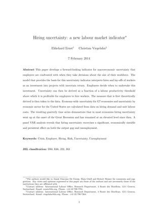
  • 16. value of a regression of productivity on time and its square. This is because the return to hiring is assumed to not follow any trend in the theoretical model. For each country and sector, we then normalize the data series in such a way that detrended productivity equals actual productivity in the first quarter of 2006. 5 Hiring uncertainty: Indicator results 5.1 Hiring uncertainty in G7 economies Hiring uncertainy calculated according to equation (34) is shown in Figures 1-7 for G7 economies. The hiring uncertainty indicator is directly compared to the policy uncertainty indicator of Baker et al. (2013) in all countries except Japan, for which policy uncertainty is not available. For now, we assume the discount factor to be constant at a level of 0.1 for all countries.13 The choice of a different discount factor that is constant over time will simply shift the uncertainty indicator upward or downwards, but does not have an impact on the fluctuations of uncertainty over time. Figure 1: Hiring uncertainty in the United States Note: Chart compares hiring uncertainty to the policy uncertainty indicator of Baker et al. (2013). Time discount factor is set to 0.1. Source: Authors’ calculations; Baker et al. (2013). Hiring uncertainty in the United States, shown in Figure 1, remained at a broadly constant level 13 In future work, we are planning to relate the discount factor to the long-term interest rate. 16
  • 17. before the Great Recession with a modest peak in 2001-2003, following the burst of the dot-com bubble and the September 11 terrorist attacks, which is also in line with the trends observed for policy uncertainty. In the end of 2007, when the Great Recession began, uncertainty has virtually jumped upwards and it has remained at high levels since then, decreasing only slowly. The decrease in hiring uncertainty is slower than the decrease in policy uncertainty that recently went back to levels observed in 2001-2003. While productivity has got back to pre-crisis levels in the meanwhile, hiring demand has not, which in the given theoretical framework is interpreted as evidence for elevated uncertainty. Figure 2: Hiring uncertainty in Canada Note: Chart compares hiring uncertainty to the policy uncertainty indicator of Baker et al. (2013). Time discount factor is set to 0.1. Source: Authors’ calculations; Baker et al. (2013). As shown in Figure 2, hiring uncertainty in Canada exhibited trends that are similar to those observed for the US. The only main difference seems that uncertainty in the beginning and mid of the 1990s was at a relatively high level in Canada which was not observed in the United States. However, the Canadian economy has seen four years of GDP growth of above 4 per cent between 1997 and 2000, which likely brought down uncertainty until the onset of the Great Recession.14 14 These data on GDP growth rates are taken from World Bank. 17
  • 18. Figure 3: Hiring uncertainty in France Note: Chart compares hiring uncertainty to the policy uncertainty indicator of Baker et al. (2013). Time discount factor is set to 0.1. Source: Authors’ calculations; Baker et al. (2013). In France, uncertainy jumped up in 2008, as illustrated in Figure 3. There have been strong fluctuations in uncertainty since then, but the level of uncertainty remains elevated. 18
  • 19. Figure 4: Hiring uncertainty in the United Kingdom Note: Chart compares hiring uncertainty to the policy uncertainty indicator of Baker et al. (2013). Time discount factor is set to 0.1. Source: Authors’ calculations; Baker et al. (2013). Even though uncertainty is not any more at its peak in the United Kingdom, as shown in Figure 4, it still is at a relatively high level compared to before the crisis. Only at the beginning of the data series, in 1992, uncertainty was at a similar level as currently. This was the last year of the beginning of the 1990s recession in the United Kingdom. Generally, it is remarkable particularly for the United Kingdom how similar the variations of hiring uncertainty and policy uncertainty are. 19
  • 20. Figure 5: Hiring uncertainty in Germany Note: Chart compares hiring uncertainty to the policy uncertainty indicator of Baker et al. (2013). Time discount factor is set to 0.1. Source: Authors’ calculations; Baker et al. (2013). In Germany, the pattern of hiring uncertainty differes from what is observed in other countries, as shown in Figure 5. Uncertainty has been on a downward trend since 2003, only interrupted by relatively small jumps upwards during the Great Recession. This trend is in line with the trend in unemployment which has been declining in the last decade, even during the Great Recession. However, the ups and downs of the series around the trend closely track the variations in policy uncertainty. 20
  • 21. Figure 6: Hiring uncertainty in Italy Note: Chart compares hiring uncertainty to the policy uncertainty indicator of Baker et al. (2013). Time discount factor is set to 0.1. Source: Authors’ calculations; Baker et al. (2013). Uncertainty in Italy has, as in most countries, increased in 2008, as Figure 6 shows. However, it has come back to lower levels in 2011, before rising again until recently. Figure 7: Hiring uncertainty in Japan Note: Time discount factor is set to 0.1. Source: Authors’ calculations. 21
  • 22. Figure 7 illustrates uncertainty in Japan which starts from a very high level in 2003, decreasing sharply until the onset of the Great Recession, before again jumping upwards to high levels in 2008 and 2009. However, in contrast to the trends observed for Canada and US, uncertainty in Japan declined again to a relatively low level between 2009 and 2013. The question arises whether uncertainty is also comparable across countries. First, we used the same discount rate for all G7 economies. In order to insure comparability across countries, this assumption needs to hold true in reality in order for uncertainty to be comparable across countries, which is somewhat difficult to verify. However, if the discount factor is assumed to be not the same, but at least similar across countries, results arguably should give a broad idea about the ranking of countries in terms of uncertainty. Second, the data that is used as an input into the uncertainty indicator has to be comparable across countries. The data on the share of firms that hires and lays off workers from the Manpower Employment Outlook Survey is comparable across countries, given that it is derived from a survey in which the same question is asked in all countries. Also the data on productivity, calculated as the inverse of unit labour costs, can be compared across countries, according to the data description by OECD. In summary, we therefore believe that our uncertainty indicator can at least to some extent be used for a cross-country comparison. Hiring uncertainty is currently at very similar levels in the United States and the United Kingdom. In Germany and Canada, hiring uncertainty is higher than in these two countries. In France, Italy and Japan, hiring uncertainty is the highest in the cross-country comparison for 2013. 5.2 Hiring uncertainty by sector in the United States Sectoral hiring uncertainy in the United States, calculated for manufacturing and construction, is shown in Figures 8-9. Once more, we assume the discount factor to be constant at a level of 0.1 in all sectors. 22
  • 23. Figure 8: Hiring uncertainty in manufacturing, United States Note: Time discount factor is set to 0.1. Source: Authors’ calculations. Hiring uncertainty in the manufacturing sector, as shown in Figure 8, broadly follows the trends observed in economy-wide uncertainty. Uncertainty in manufacturing went up at the onset of the Great Recession and was on a declining trend between mid of 2009 and 2011. In contrast to the economy-wide indicator, however, hiring uncertainty in manufacturing went down much stronger, almost reaching pre-crisis levels already in 2011. 23
  • 24. Figure 9: Hiring uncertainty in construction, United States Note: Time discount factor is set to 0.1. Source: Authors’ calculations. Hiring uncertainty in the construction sector, shown in Figure 9, was trending upwards between 2007 and 2011, the whole period for which the indicator is available. Only in 2007 and 2011, there were few quarters in which uncertainty did not increase. The upward trend in uncertainty within the construction sector is consistent with the many jobs lost in that sector during the crisis. 6 How does hiring uncertainty affect growth and jobs? Hiring uncertainty is expected to have an effect on employment dynamics, separate and distinct from overall macroeconomic conditions such as output growth. The heightened uncertainty that companies face on labour markets will make them reluctant to open new vacancies and give them incentives to shed more workers, thereby pushing up unemployment rates. At the same time, higher hiring uncertainty is an indication of a generally weak macroeconomic environment, holding back companies’ investment and thereby lowering GDP growth. In this section, we analyse the importance and pass-through of this effect and compare it with effects such as those generated by policy uncertainty. The analysis of the uncertainty pass-through is based on a 3-variables vector-autoregression system 24
  • 25. Figure 10: Summary of VAR results WĂŶĞů KƵƚƉƵƚ ŐĂƉ hŶĞŵƉůŽLJŵĞŶƚ ,ŝƌŝŶŐ ƵŶĐĞƌƚĂŝŶƚLJ KƵƚƉƵƚ ŐĂƉ h^ hŶĞŵƉůŽLJŵĞŶƚ ,ŝƌŝŶŐ ƵŶĐĞƌƚĂŝŶƚLJ KƵƚƉƵƚ ŐĂƉ KƵƚƉƵƚ ŐĂƉ ĂŶĂĚĂ KƵƚƉƵƚ ŐĂƉ hŶĞŵƉůŽLJŵĞŶƚ ,ŝƌŝŶŐ ƵŶĐĞƌƚĂŝŶƚLJ KƵƚƉƵƚ ŐĂƉ hŶĞŵƉůŽLJŵĞŶƚ ,ŝƌŝŶŐ ƵŶĐĞƌƚĂŝŶƚLJ KƵƚƉƵƚ ŐĂƉ hŶĞŵƉůŽLJŵĞŶƚ hŶĞŵƉůŽLJŵĞŶƚ hŶĞŵƉůŽLJŵĞŶƚ ,ŝƌŝŶŐ ƵŶĐĞƌƚĂŝŶƚLJ ,ŝƌŝŶŐ ƵŶĐĞƌƚĂŝŶƚLJ ,ŝƌŝŶŐ ƵŶĐĞƌƚĂŝŶƚLJ h KƵƚƉƵƚ ŐĂƉ hŶĞŵƉůŽLJŵĞŶƚ ,ŝƌŝŶŐ ƵŶĐĞƌƚĂŝŶƚLJ KƵƚƉƵƚ ŐĂƉ KƵƚƉƵƚ ŐĂƉ ƌĂŶĐĞ hŶĞŵƉůŽLJŵĞŶƚ ,ŝƌŝŶŐ ƵŶĐĞƌƚĂŝŶƚLJ KƵƚƉƵƚ ŐĂƉ 'ĞƌŵĂŶLJ KƵƚƉƵƚ ŐĂƉ hŶĞŵƉůŽLJŵĞŶƚ hŶĞŵƉůŽLJŵĞŶƚ hŶĞŵƉůŽLJŵĞŶƚ ,ŝƌŝŶŐ ƵŶĐĞƌƚĂŝŶƚLJ ,ŝƌŝŶŐ ƵŶĐĞƌƚĂŝŶƚLJ ,ŝƌŝŶŐ ƵŶĐĞƌƚĂŝŶƚLJ /ƚĂůLJ KƵƚƉƵƚ ŐĂƉ hŶĞŵƉůŽLJŵĞŶƚ ,ŝƌŝŶŐ ƵŶĐĞƌƚĂŝŶƚLJ KƵƚƉƵƚ ŐĂƉ KƵƚƉƵƚ ŐĂƉ :ĂƉĂŶ hŶĞŵƉůŽLJŵĞŶƚ ,ŝƌŝŶŐ ƵŶĐĞƌƚĂŝŶƚLJ KƵƚƉƵƚ ŐĂƉ hŶĞŵƉůŽLJŵĞŶƚ hŶĞŵƉůŽLJŵĞŶƚ ,ŝƌŝŶŐ ƵŶĐĞƌƚĂŝŶƚLJ ,ŝƌŝŶŐ ƵŶĐĞƌƚĂŝŶƚLJ as follows:         Gapt,j U nrt,j U ncertaintyt,j   =    Gapt−i,j 4     i=1  Note: The chart displays the result of a 3x3 VAR including the output gap, the unemployment rate and the ILO hiring uncertainty index. The VAR includes four lags of each variable. The size of the pies correspond to the sum of the coefficients, a red pie indicates a negative sum, a blue pie stands for a positive sign. Source: ILO Hiring uncertainty indicator; OECD Economic Outlook database 94; own calculations. U nrt−i,j U ncertaintyt−i,j    + αj + εt,j   where gapt : the output gap measured using HP-filtered GDP growth, U nrt : the (HP-filtered) unemployment rate, U ncertaintyt : our preferred measure of hiring uncertainty as discussed in the previous section and α: a constant/fixed effect. We use quarterly data and a lag structure of the last 4 quarters. The VAR is estimated for each of our seven economies individually (hence dropping the country index j) as well as in a panel, using αj fixed effects to distinguish between the countries. The following figure 10 gives an overview of the sum of coefficients for the different estimated equations both for the panel and for individual countries. As the figure indicates, all coefficient sums have the expected signs - hiring uncertainty lowers output and increases unemployment - but with variations in the quantitative importance for individual countries and in comparison to the panel as a whole. The results are robust to changes in specification such as a change in the number of lags or the use of alternative measures of GDP and employment - e.g. using GDP growth rather than the output gap or using employment growth rather than the unemployment rate. In contrast, using alternative measures of uncertainty - such as 25
  • 26. the policy uncertainty index by Baker et al. (2013), or a measure of implied volatility on the labour market - can substantially change the results of the estimation, at least for individual countries if not for the panel overall.15 To further analyse the pass-through and better understand how hiring uncertainty affects the labour market, we added more detail to the above model using the ILO’s Quarterly Labour Flows database. This allowed us to differentiate between unemployment inflows - a proxy measure for job destruction - and unemployment outflows - a proxy measure for job creation - in the above VAR:  Gapt,j    U nInf lowst,j     U nOutf lowst,j  U ncertaintyt,j       =    Gapt−i,j    U nInf lowst−i,j    i=1  U nOutf lowst−i,j  U ncertaintyt−i,j 4       + αj + εt,j    (35) where instead of the unemployment rate we now distinguish between U nInf lowst : the unemployment inflows and U nOutf lowst : the unemployment outflows. As in Ernst and Rani (2011), we assume that unemployment inflows and outflows are not independent from each other but rather exercise a mutual influence. The shock pass-through is now analysed by imposing a structure on the shock structure, using a Choleski decomposition of the error matrix. Using the above ordering of the variables, we assume that hiring uncertainty is the most exogenous shock, whereas the output gap is the most endogenous one. The corresponding SVAR then yields the following impulse-response function(s) for the four different shocks, differentiating between country-individual estimations and the panel as a whole. As figure 11 demonstrates, hiring uncertainty has a strong effect on the output gap but which runs only partially through changes in unemployment outflows. Rather, it is unemployment inflows, i.e. job destruction, that are most affected by shocks to hiring uncertainty (panel 4). On the other hand, shocks to unemployment outflows reduce hiring uncertainty for an extended period of time (up to 10 quarters), at least when the panel as a whole is considered (panel 3). Finally, demand shocks such as those that drive the output gap have strong, but short-lived effects on hiring uncertainty as much as they influence the dynamics on the labour market directly (panel 1). 15 For an overview of the VAR results using different uncertainty measures see the figures in the annex section. Detailed regression results of the base specification and alternative indicators and set-ups are available from the authors upon request. 26
  • 27. Figure 11: Impulse-responses with structural shocks Response to structural shock #1 −4 Output gap Response to structural shock #2 Unemployment inflows x 10 0.8 −4 Output gap 2 Unemployment inflows x 10 0.2 0.6 8 0 0.4 0 0.2 6 −2 4 −0.2 0 2 −4 −0.2 −0.4 −0.4 0 −6 5 −3 10 15 20 5 10 Unemployment outflows x 10 15 −2 20 5 Hiring uncertainty −3 8 20 0 10 15 20 0.02 2 0.01 1 4 5 Hiring uncertainty 3 0.01 6 15 Unemployment outflows x 10 10 10 −0.01 0 2 −0.02 0 −0.03 5 10 United States 15 Canada −0.01 −2 −2 Panel 0 −1 20 5 United Kingdom 10 France 15 Germany −3 20 Italy 5 Panel Japan 10 United States 15 Canada Response to structural shock #3 Unemployment inflows x 10 0.4 5 10 France 15 Germany 20 Italy Japan Response to structural shock #4 −4 Output gap 20 United Kingdom −4 Output gap Unemployment inflows x 10 2 3 0.1 0.2 2 1 0 1 0 0 −0.1 0 −1 −0.2 −0.2 −1 −2 −0.4 −0.3 5 −3 10 15 20 5 Unemployment outflows x 10 10 15 −2 20 5 −3 Hiring uncertainty 10 15 20 5 Unemployment outflows x 10 10 15 20 Hiring uncertainty 4 10 0.02 −5 −2 United States 10 15 Canada 20 United Kingdom 0.04 0.02 0 −4 −0.04 5 Panel 0 −0.02 0 0.06 2 0 5 5 France 10 Germany 15 20 Italy 5 Japan Panel United States 10 15 Canada 20 United Kingdom 5 France 10 Germany 15 20 Italy Japan Note: The chart displays the impulse-response functions for the four structural shocks based on equation (35). The four shocks are #1: a shock on the output gap, #2: a shock on unemploment inflows, #3: a shock on unemployment outflows, #4: a shock on hiring uncertainty. 7 Conclusion This paper derives a measure for the macroeconomic uncertainty that employers are confronted with when taking decisions about the size of their workforce. As theoretical framework, the paper adapts the investment model of McDonald and Siegel (1986) to the context of hires and lay-offs and interprets employers’ changes in the size of the workforce as investment decisions. Employers have to decide when to hire or layoff workers. The result of the model indicates that the expected return to hiring needs to be strictly larger than the costs in order to make it optimal for employers to hire at a given point of time. The size of the difference between the expected return and the costs depends on the level of uncertainty in the market. Based on the model, we can derive two productivity thresholds that mark the levels of labour productivity above which firms hire workers and below which firms lay workers off. Assuming productivity to be distributed log-normally across firms, we then derive uncertainty as a function of the shares of firms that intend to hire workers and lay workers off as well as the average labour productivity in the economy or sector. Using data on average labour productivity 27
  • 28. from OECD and on firms’ hiring and lay-off intentions from the ManpowerGroup, we calculate uncertainty indicators for G7 countries as well as sectoral uncertainty for the United States. For most countries, hiring uncertainty follows quite similar trends as the policy uncertainty indicator of Baker et al. (2013), which gives us some confidence in the validity of our approach. However, there also differences which remain to be examined in more detail. Our hiring uncertainty indicator displays important correlation with both unemployment and the output gap, over and above the direct link between labour market and demand variables. Our indicator is robust to specification changes and shows more regularity in its impact across countries than alternative uncertainty indicators. A more detailed analysis of the pass-through of uncertainty shocks reveals that job destruction is a key channel through which hiring uncertainty affects labour market dynamics and the output gap. Future work will also focus on a broadening of the indicator coverage with respect to countries and economic sectors. In particular, we aim at developing a measure for hiring uncertainty also for emerging and developing economies, which should be feasible for some countries, given that data on hiring intentions and unit labour costs are available. Moreover, we intend to examine the factors that have an impact on hiring uncertainty and analyze the role that hiring uncertainty can play to improve unemployment forecasts. 28
  • 29. References Altomonte, C.; Aquilante, T.; Ottaviano, G. 2012. The Triggers of Competitiveness: The EFIGE Cross-country Report, Bruegel Blueprint Series (Brussels, Bruegel). Baker, S.; Bloom, N.; Davis, S. 2013. “Measuring Economic Policy Uncertainty”, Paper published on http://www.policyuncertainty.com. Baum, C. et al. 2006. “The Impact of Macroeconomic Uncertainty on Non-Financial Firms’ Demand for Liquidity”, in Review of Financial Economics, vol. 15, pp. 289–304. Bloom, N. et al. 2012. “Really Uncertain Business Cycles”, NBER Working Paper 18245, Cambridge (MA): National Bureau of Economic Research. Dixit, A.; Pindyck, R. 1994. Investment Under Uncertainty (Princeton, Princeton University Press). Dosi, G.; Lei, J.; Yu, X. 2013. “Institutional Change and Productivity Growth in China’s Manufacturing 1998-2007: The Microeconomics of Creative Restructuring”, LEM Working Paper Series 2013/07, Pisa: Laboratory of Economics and Management. Ernst, E.; Rani, U. 2011. “Understanding unemployment flows”, in Oxford Review of Economic Policy, vol. 27, no. 2, pp. 268–294. Haddow, A. et al. 2013. “Macroeconomic Uncertainty: What is it, How can we Measure it and Why Does it Matter?”, in Quarterly Bulletin (Bank of England), vol. 2013Q2, pp. 100–109. ILO. 2013a. Global Employment Trends 2013: Recovering from a Second Jobs Dip (Geneva, International Labour Office). —. 2013b. “The ILO Estimates on Unemployment Flows: Introducing Flows to Assess the Variations in Unemployment”, in Key Indicators of the Labour Market, 8th edition (Geneva, International Labour Office). McDonald, R.; Siegel, D. 1986. “The Value of Waiting to Invest”, in Quarterly Journal of Economics, vol. 101, no. 4, pp. 707–728. Melitz, M. 2003. “The Impact of Trade on Intra-Industry Reallocations and Aggregate Industry Productivity”, in Econometrica, vol. 71, no. 6, pp. 1695–1725. 29
  • 30. Morissette, R.; Lu, Y.; Qiu, T. 2013. “Worker Reallocation in Canada”, Analytical Studies Branch Research Paper Series no. 348, Ottawa: Statistics Canada. Okubo, T.; Tomiura, E. 2013. “Productivity Distribution, Firm Heterogeneity and Agglomeration: Evidence from Firm-level Data”, RIETI Discussion Paper Series 10-E-017, Tokyo: The Research Institute of Economy, Trade and Industry. 30
  • 31. Annex figures Figure 12: Summary of VAR results: Policy uncertainty WĂŶĞů KƵƚƉƵƚ ŐĂƉ hŶĞŵƉůŽLJŵĞŶƚ ,ŝƌŝŶŐ ƵŶĐĞƌƚĂŝŶƚLJ h^ KƵƚƉƵƚ ŐĂƉ hŶĞŵƉůŽLJŵĞŶƚ ,ŝƌŝŶŐ ƵŶĐĞƌƚĂŝŶƚLJ KƵƚƉƵƚ ŐĂƉ KƵƚƉƵƚ ŐĂƉ ĂŶĂĚĂ KƵƚƉƵƚ ŐĂƉ hŶĞŵƉůŽLJŵĞŶƚ ,ŝƌŝŶŐ ƵŶĐĞƌƚĂŝŶƚLJ KƵƚƉƵƚ ŐĂƉ hŶĞŵƉůŽLJŵĞŶƚ ,ŝƌŝŶŐ ƵŶĐĞƌƚĂŝŶƚLJ KƵƚƉƵƚ ŐĂƉ hŶĞŵƉůŽLJŵĞŶƚ hŶĞŵƉůŽLJŵĞŶƚ hŶĞŵƉůŽLJŵĞŶƚ ,ŝƌŝŶŐ ƵŶĐĞƌƚĂŝŶƚLJ ,ŝƌŝŶŐ ƵŶĐĞƌƚĂŝŶƚLJ ,ŝƌŝŶŐ ƵŶĐĞƌƚĂŝŶƚLJ h KƵƚƉƵƚ ŐĂƉ hŶĞŵƉůŽLJŵĞŶƚ ,ŝƌŝŶŐ ƵŶĐĞƌƚĂŝŶƚLJ KƵƚƉƵƚ ŐĂƉ ƌĂŶĐĞ KƵƚƉƵƚ ŐĂƉ hŶĞŵƉůŽLJŵĞŶƚ ,ŝƌŝŶŐ ƵŶĐĞƌƚĂŝŶƚLJ KƵƚƉƵƚ ŐĂƉ 'ĞƌŵĂŶLJ KƵƚƉƵƚ ŐĂƉ hŶĞŵƉůŽLJŵĞŶƚ hŶĞŵƉůŽLJŵĞŶƚ hŶĞŵƉůŽLJŵĞŶƚ ,ŝƌŝŶŐ ƵŶĐĞƌƚĂŝŶƚLJ ,ŝƌŝŶŐ ƵŶĐĞƌƚĂŝŶƚLJ ,ŝƌŝŶŐ ƵŶĐĞƌƚĂŝŶƚLJ /ƚĂůLJ KƵƚƉƵƚ ŐĂƉ hŶĞŵƉůŽLJŵĞŶƚ Note: The chart displays the result of a 3x3 VAR including the output gap, the unemployment rate and Baker’s policy uncertainty index. The VAR includes four lags of each variable. The size of the pies correspond to the sum of the coefficients, a red pie indicates a negative sum, a blue pie stands for a positive sign. Source: Baker et al. (2013); OECD Economic Outlook database 94; own calculations. ,ŝƌŝŶŐ ƵŶĐĞƌƚĂŝŶƚLJ KƵƚƉƵƚ ŐĂƉ hŶĞŵƉůŽLJŵĞŶƚ ,ŝƌŝŶŐ ƵŶĐĞƌƚĂŝŶƚLJ Figure 13: Summary of VAR results: Implicit volatility WĂŶĞů KƵƚƉƵƚ ŐĂƉ hŶĞŵƉůŽLJŵĞŶƚ ,ŝƌŝŶŐ ƵŶĐĞƌƚĂŝŶƚLJ h^ KƵƚƉƵƚ ŐĂƉ hŶĞŵƉůŽLJŵĞŶƚ ,ŝƌŝŶŐ ƵŶĐĞƌƚĂŝŶƚLJ KƵƚƉƵƚ ŐĂƉ KƵƚƉƵƚ ŐĂƉ ĂŶĂĚĂ KƵƚƉƵƚ ŐĂƉ hŶĞŵƉůŽLJŵĞŶƚ ,ŝƌŝŶŐ ƵŶĐĞƌƚĂŝŶƚLJ KƵƚƉƵƚ ŐĂƉ hŶĞŵƉůŽLJŵĞŶƚ ,ŝƌŝŶŐ ƵŶĐĞƌƚĂŝŶƚLJ KƵƚƉƵƚ ŐĂƉ hŶĞŵƉůŽLJŵĞŶƚ hŶĞŵƉůŽLJŵĞŶƚ hŶĞŵƉůŽLJŵĞŶƚ ,ŝƌŝŶŐ ƵŶĐĞƌƚĂŝŶƚLJ ,ŝƌŝŶŐ ƵŶĐĞƌƚĂŝŶƚLJ ,ŝƌŝŶŐ ƵŶĐĞƌƚĂŝŶƚLJ h KƵƚƉƵƚ ŐĂƉ hŶĞŵƉůŽLJŵĞŶƚ ,ŝƌŝŶŐ ƵŶĐĞƌƚĂŝŶƚLJ KƵƚƉƵƚ ŐĂƉ ƌĂŶĐĞ KƵƚƉƵƚ ŐĂƉ hŶĞŵƉůŽLJŵĞŶƚ ,ŝƌŝŶŐ ƵŶĐĞƌƚĂŝŶƚLJ KƵƚƉƵƚ ŐĂƉ 'ĞƌŵĂŶLJ KƵƚƉƵƚ ŐĂƉ hŶĞŵƉůŽLJŵĞŶƚ hŶĞŵƉůŽLJŵĞŶƚ hŶĞŵƉůŽLJŵĞŶƚ ,ŝƌŝŶŐ ƵŶĐĞƌƚĂŝŶƚLJ ,ŝƌŝŶŐ ƵŶĐĞƌƚĂŝŶƚLJ ,ŝƌŝŶŐ ƵŶĐĞƌƚĂŝŶƚLJ /ƚĂůLJ KƵƚƉƵƚ ŐĂƉ KƵƚƉƵƚ ŐĂƉ hŶĞŵƉůŽLJŵĞŶƚ ,ŝƌŝŶŐ ƵŶĐĞƌƚĂŝŶƚLJ :ĂƉĂŶ KƵƚƉƵƚ ŐĂƉ hŶĞŵƉůŽLJŵĞŶƚ KƵƚƉƵƚ ŐĂƉ hŶĞŵƉůŽLJŵĞŶƚ hŶĞŵƉůŽLJŵĞŶƚ ,ŝƌŝŶŐ ƵŶĐĞƌƚĂŝŶƚLJ ,ŝƌŝŶŐ ƵŶĐĞƌƚĂŝŶƚLJ 31 ,ŝƌŝŶŐ ƵŶĐĞƌƚĂŝŶƚLJ Note: The chart displays the result of a 3x3 VAR including the output gap, the unemployment rate and the ILO implicit labour market volatility index. The VAR includes four lags of each variable. The size of the pies correspond to the sum of the coefficients, a red pie indicates a negative sum, a blue pie stands for a positive sign. Source: ILO Implicit labour market volatility ; OECD Economic Outlook database 94; own calculations.