
Recommended
Recommended
More Related Content
What's hot
What's hot (8)
Similar to 01 matrices
Similar to 01 matrices (16)
Recently uploaded
Recently uploaded (20)
01 matrices
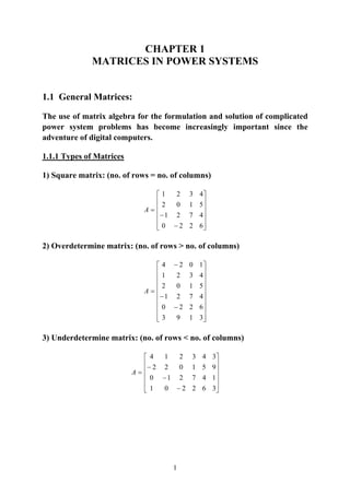
- 1. 1 CHAPTER 1 MATRICES IN POWER SYSTEMS 1.1 General Matrices: The use of matrix algebra for the formulation and solution of complicated power system problems has become increasingly important since the adventure of digital computers. 1.1.1 Types of Matrices 1) Square matrix: (no. of rows = no. of columns) ⎥ ⎥ ⎥ ⎥ ⎦ ⎤ ⎢ ⎢ ⎢ ⎢ ⎣ ⎡ − − = 6220 4721 5102 4321 A 2) Overdetermine matrix: (no. of rows > no. of columns) ⎥ ⎥ ⎥ ⎥ ⎥ ⎥ ⎥ ⎥ ⎦ ⎤ ⎢ ⎢ ⎢ ⎢ ⎢ ⎢ ⎢ ⎢ ⎣ ⎡ − − − = 3193 6220 4721 5102 4321 1024 A 3) Underdetermine matrix: (no. of rows < no. of columns) ⎥ ⎥ ⎥ ⎥ ⎦ ⎤ ⎢ ⎢ ⎢ ⎢ ⎣ ⎡ − − − = 362201 147210 951022 343214 A
- 2. 2 4) Upper triangular matrix: (aij = 0 for all i > j) ⎥ ⎥ ⎥ ⎥ ⎦ ⎤ ⎢ ⎢ ⎢ ⎢ ⎣ ⎡ = 6000 4700 5100 4321 A 5) Lower triangular matrix: (aij = 0 for all i < j) ⎥ ⎥ ⎥ ⎥ ⎦ ⎤ ⎢ ⎢ ⎢ ⎢ ⎣ ⎡ − = 7000 0721 0002 0001 A 6) Diagonal matrix: (aij = 0 for all i ≠ j) ⎥ ⎥ ⎥ ⎥ ⎦ ⎤ ⎢ ⎢ ⎢ ⎢ ⎣ ⎡ − = 7000 0700 0080 0001 A 7) Unit (U) or Identity (I) matrix: (aij = 0 for all i ≠ j & aij = 1 for all i = j) ⎥ ⎥ ⎥ ⎥ ⎦ ⎤ ⎢ ⎢ ⎢ ⎢ ⎣ ⎡ = 1000 0100 0010 0001 A 1.1.2 Special Matrices 1) Null if A = A ⎥ ⎥ ⎥ ⎥ ⎦ ⎤ ⎢ ⎢ ⎢ ⎢ ⎣ ⎡ = 0000 0000 0000 0000 A 2) Symmetric if A = At
- 3. 3 ⎥ ⎥ ⎥ ⎥ ⎦ ⎤ ⎢ ⎢ ⎢ ⎢ ⎣ ⎡ = 6454 4713 5102 4321 A 3) Skew-Symmetric if - A = At ⎥ ⎥ ⎥ ⎥ ⎦ ⎤ ⎢ ⎢ ⎢ ⎢ ⎣ ⎡ − − − −−− = 0454 4013 5102 4320 A 4) Real if A = A* ⎥ ⎥ ⎥ ⎥ ⎦ ⎤ ⎢ ⎢ ⎢ ⎢ ⎣ ⎡ ++−−+ +++−− ++++ ++++ = 06020200 04070201 05010002 04030201 jjjj jjjj jjjj jjjj A 5) Pure-imaginary if A = -A* ⎥ ⎥ ⎥ ⎥ ⎦ ⎤ ⎢ ⎢ ⎢ ⎢ ⎣ ⎡ ++−+ +++− ++++ ++++ = 60202000 40702010 50100020 40302010 jjjj jjjj jjjj jjjj A 6) Hermition if A = (A* )t ⎥ ⎥ ⎥ ⎥ ⎦ ⎤ ⎢ ⎢ ⎢ ⎢ ⎣ ⎡ +−++ +++− −−++ −+−+ = 06445544 44071133 55110022 44332201 jjjj jjjj jjjj jjjj A 7) Skew-Hermition if A = -(A* )t ⎥ ⎥ ⎥ ⎥ ⎦ ⎤ ⎢ ⎢ ⎢ ⎢ ⎣ ⎡ +−−−+ +−−− −−+ +−−−+− = 0445544 4401133 5511022 4433220 jjj jjj jjj jjj A
- 4. 4 8) Orthogonal if Qt Q = I ⎥ ⎥ ⎥ ⎥ ⎦ ⎤ ⎢ ⎢ ⎢ ⎢ ⎣ ⎡ −− −− −− = 2835.06157.05519.04858.0 3040.02291.06650.06425.0 6122.04734.04966.03931.0 6726.05868.00812.04434.0 Q (where Q is an orthonormal basis for the range of the square matrix A) 9) Unitary if (A* )t A = U ⎥ ⎥ ⎥ ⎦ ⎤ ⎢ ⎢ ⎢ ⎣ ⎡ +−−− −−+−= 35.05.035.05.01 35.05.035.05.01 111 3 1 jj jjA References: [1] G.W. Stagg and A.H. El-Abiad, "Computer Methods in Power System Analysis", McGraw-Hill, New York, 1968.