Lasso and ridge regression

2. The equation of a straight line is
 b = value of y when x=0 (intercept)
 m = Slope or Gradient (how steep the line is)
Reference: https://www.mathsisfun.com/equation_of_line.html

3. Linear regression is an approach to model the relationship between a dependent variable and one
or more independent variables.
 Linear Regression model try to create a linear
relationship between dependent (salary) and
independent (experience) variables.
 It try to create the equation of a straight line (salary =
m * experience + b) with minimum error (residual)
between actual value and predicted value.
 Equation for simple linear regression : y = m*x + b
 Equation for multiple linear regression : y = m1*x1 + m2*x2 + …. + mn*xn + b
Linear Regression tries to create best fit line with minimum
sum of residuals (∑ ( Y – Ypredict )^2) which is also known as
cost function.

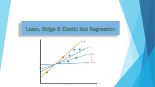
4. Slope = 1
Intercept = 0
Slope = 0
Intercept = 0
Slope =
Undefined (1/0)
 In case of the lines having higher slope, any
minor variation in x can cause to a major
variation in y.
 In the linear regression model creating with
such data can have overfitting problem.
 One solution is to penalize the slopes and
make the model a generalized one.
 LASSO and RIDGE regression are models will
help for the same.
Underfitting occurs when a model can’t accurately
capture the dependencies among data, usually as a
consequence of its own simplicity. It often yields a
with known data and bad generalization
applied with new data.
Overfitting happens when a model learns both
dependencies among data and random
words, a model learns the existing data too well.
models usually yield high 𝑅². However, they often
generalize well and have significantly lower 𝑅²
with new data.

5. A good way to reduce overfitting is to regularize the model (i.e.,
to constrain it):
For a linear model, regularization is typically achieved by
constraining the weights of the model. Why?
The size of coefficients increase exponentially with increase in model
complexity
Techniques like Ridge Regression, Lasso Regression, and
Elastic Net, implement three different ways to constrain the
weights.

6. Least Absolute Shrinkage and Selection
Operator Regression (simply called Lasso
Regression) is another regularized version of
Linear Regression: that adds a L1
regularization term to the cost function,
The minimization objectives is MSE +  * | m |
Default value of alpha is 1. It can be zero to any positive
number.
Lasso Regression tends to completely
eliminate the weights of the least important
features (i.e., set them to zero).

7. Ridge Regression (also called Tikhonov
regularization) is a L2 regularized version of Linear
Regression: a regularization term equal to  *
slope^2 is added to the cost function.
The minimization objectives is MSE +  * m^2
This forces the learning algorithm to not only fit
the data but also keep the model weights as small
as possible.
Note that the regularization term should only be
added to the cost function during training.
The  (alpha) balance the amount of emphasis to the
regularization. Default value of alpha is 1. It can be
zero to any positive number.
 = 0  simple linear regression
 =   all coefficients become zero
increasing α leads to flatter (i.e., less extreme,
more reasonable) predictions.

8. Elastic net is a popular type of regularized linear regression that combines
two popular penalties, specifically the L1 and L2 penalty functions.
Similar to Ridge and LASSO Elastic Net is an extension of linear regression,
this adds regularization penalties to the loss function during training.
The penalty is a mixture of L1 and L2 penalties. Alpha and l1_ratio arguments
decides the same. Default value of alpha is 1 and can be passed according to
convenience of the data.
l1_ratio can have value from 0 to 1. Default value =0.5. l1_ratio = 0 means the
penalty is an L2 penalty. l1_ratio = 1 means it is an L1 penalty. l1_ratio is
between 0 and 1, the penalty is a combination of L1 and L2.
Reference: https://machinelearningmastery.com/elastic-net-regression-in-python/