Matrices

1. 2- 1
Chapter 2 Matrices
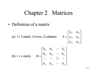
• Definition of a matrix












32
31
22
21
12
11
A
columns)
2
rows,
(3
matrix
2
3
(a)
a
a
a
a
a
a














rc
r
r
c
c
b
b
b
b
b
b
b
b
b









2
1
2
22
21
1
12
11
B
matrix
c
r
(b)

2. 2- 2
6
4
24
-
3
4
24
3
4
1
2
2
1
1
3
2
1
1
3
2
1
E
PL
d
L
E
wL
d
L
E
wL
d
L















A system of 3 equations:
Represented by a matrix:






















1
2
1
3
1
3
6
4
1
1
24
3
4
1
24
3
1
4
E
PL
L
E
wL
L
E
wL
L

3. 2- 3
Types of Matrices
• Square matrix: # of rows = # of columns
• upper triangular matrix strictly upper triangular matrix










33
32
31
23
22
21
13
12
11
a
a
a
a
a
a
a
a
a
0
0
0
0
0
0
0
0
0
0
55
45
44
35
34
33
25
24
23
22
15
14
13
12
11
















a
a
a
a
a
a
a
a
a
a
a
a
a
a
a
0
0
0
0
0
0
0
0
0
0
0
0
0
0
0
45
35
34
25
24
23
15
14
13
12
















a
a
a
a
a
a
a
a
a
a

4. 2- 4
• lower triangular matrix strictly lower triangular matrix
• diagonal matrix
0
0
0
0
0
0
0
0
0
0
55
54
53
52
51
44
43
42
41
33
32
31
22
21
11
















a
a
a
a
a
a
a
a
a
a
a
a
a
a
a
0
0
0
0
0
0
0
0
0
0
0
0
0
0
0
54
53
52
51
43
42
41
32
31
21
















a
a
a
a
a
a
a
a
a
a
0
0
0
0
0
0
0
0
0
0
0
0
n
1
2
1
































5. 2- 5
• banded matrix
a square matrix with elements of zero except for the principal
diagonal and values in the positions adjacent to the diagonal.
• tridiagonal matrix
0
0
0
0
0
0
0
0
0
0
0
0
55
54
45
44
43
34
33
32
23
22
21
12
11
















a
a
a
a
a
a
a
a
a
a
a
a
a

6. 2- 6
• unit matrix: 1 on the principal diagonal
• null matrix: All elements are zero.
1
0
0
0
0
0
1
0
0
0
0
0
1
0
0
0
0
0
1
0
0
0
0
0
1

















Ι
0
0
0
0
0
0
0
0
0
0
0
0
0
0
0
0
0
0
0
0
0
0
0
0
0

















O

7. 2- 7
• symmetric matrix:
a square matrix in which
• skew-symmetric matrix:
a square matrix in which for all i
and j
ji
ij a
a 
1.00
0.64
0.27
-
0.64
1.00
0.23
-
0.27
-
0.23
-
1.00










ji
ij a
a 


8. 2- 8
• transpose of matrix A: AT
• (AT) T = A
ji
T
ij a
a 




























5
.
6
3
.
8
4
.
6
1
.
7
7
.
7
55
188
53
12
35
60
132
283
195
140
5
.
6
55
60
3
.
8
188
132
4
.
6
53
283
1
.
7
12
195
7
.
7
35
140
T
A
A

9. 2- 9
Matrix Operations
• Matrix equality
• Matrix addition and subtraction
C = A + B = B + A (commutative)
C = A - B
ij
ij
ij b
a
c 

ij
ij
ij b
a
c 

j
i
b
a ij
ij and
all
for
if 
 B
A

10. 2- 10
• Example: Matrix addition and subtraction
11
10
9
5
3
1
6
4
2











A
1
1
2
4
8
7
3
2
0











B
12
11
11
9
11
8
9
6
2












 B
A
C















10
9
7
1
5
6
3
2
2
B
A
D

11. 2- 11
Matrix Multiplication
• One example
81
43
55
35
4(9)
8(3)
3(7)
4(3)
8(2)
3(5)
1(9)
6(3)
4(7)
)
3
(
1
)
2
(
6
)
5
(
4
9
3
3
2
7
5
4
8
3
1
6
4









































 C
S
T

12. 2- 12
Rules of Matrix Multiplication
1. # of columns in A = # of rows in B
2. # of rows in C = # of rows in A
3. # of columns in C = # of columns in B
4.
B
A
C 




m
k
kj
ik
ij b
a
c
1

13. 2- 13
5. Matrix multiplication is not commutative
6. Matrix multiplication is associative
A
B
B
A 


)
(
)
)
( C
B
A
C
B
A 





14. 2- 14
Example: Matrix Multiplication











11
10
9
5
3
1
6
4
2
A











1
1
2
4
8
7
3
2
0
B
78
109
92
20
31
31
28
42
40












 B
A
E
28
21
14
126
92
58
43
36
29












 A
B
F
A
B
B
A 



15. 2- 15
Matrix Multiplication by a Scalar
ij
ij sa
b
s 
 A
B
10
11
10
9
5
3
1
6
4
2











 s
A












110
100
90
50
30
10
60
40
20
A
B s
An example:

16. 2- 16
Matrix Inversion
where A-1 is the inverse of A, and I is the
unit matrix
I
A
A 1



1
c
0
c
0
c
1
c
22
22
12
21
21
22
11
21
22
12
12
11
21
12
11
11








a
c
a
a
c
a
a
c
a
a
c
a
equations
us
simultaneo
following
by the
determined
be
can
inverse
the
,
)
(
and
2
If
2
n
c
n ij

 1
A

17. 2- 17
Example: Matrix Inversion




















1
0
0
1
7
5
3
2
22
21
12
11
c
c
c
c







7
5
3
2
A
1
7
3
0
5
2
0
7
3
1
5
2
22
21
22
21
12
11
12
11








c
c
c
c
c
c
c
c










2
5
3
7
get
we
1
A

18. 2- 18
Matrix Singularity
• If the inverse of a matrix A exists, then A is
said to be nonsingular.
• If the inverse of a matrix A does not exist,
then A is said to be singular.
• If matrix A is singular, then the linear
system of simultaneous equations
represented by A has no unique solution.

19. 2- 19
There are an infinite number of solutions if 2a = b.
There is no feasible solution if 2a  b.
Thus matrix A is singular.
b
X
X
a
X
X




2
1
2
1
6
4
3
2
6
4
3
2
Let 






A




















1
0
0
1
6
4
3
2
for
solution
No
22
21
12
11
c
c
c
c

20. 2- 20
• trace of a square matrix = sum of diagonal elements
• matrix augmentation: addition of a column or columns
to the initial matrix



n
i
ii
a
tr
1
)
(A
1
0
0
0
1
0
0
0
1
4
3
2
1
4
1
1
3
2
4
3
2
1
4
1
1
3
2





















 a
A
A

21. 2- 21
• matrix partition







22
21
12
11
A
A
A
A
A
4
3
2
1
4
1
1
3
2











A
   
4
3
2
1
1
4
1
3
2
















22
21
12
11
A
A
A
A

22. 2- 22
Vectors
• Column vector
• Row vector
• Vectors of two ordinates
 
1
3
2










2
1
2

23. 2- 23
• orthogonal vectors
Two vectors are said to be orthogonal if their product
is equal to zero.
If two vector are orthogonal, they are perpendicular to
each other in the n-dimensional space.
   
0
1
3
2
example,
For
3
2 









24. 2- 24
5
0
1
2
length
vector
.
n
i
i )
v
( 


• normalized vectors
A vector is normalized by dividing each element by its
length.
A normalized vector has a length 1.
Two vectors that are both normalized and orthogonal to
each other are said to be orthonormal vectors.

25. 2- 25
Example: Vectors
5]
3
-
[2
1 
V
1
1
1
2











V
6.164
38
)
5
(
)
3
(
(2)
of
length 2
2
2
1 





V
732
.
1
3
)
1
(
)
1
(
(-1)
of
length 2
2
2
2 




V

26. 2- 26





 

38
5
38
3
38
2
1n
V





 

3
1
3
1
3
1
2n
V
Normalized vectors:
l.
orthonorma
are
and
.
orthogonal
are
and
,
0
Since
2
1
1
1
n
n V
V
V
V
V
V 2
2 


27. 2- 27
Determinants
• A determinant of a matrix A is denoted by |A|.
• The determinant of a 22 matrix:
• The determinant of a 33 matrix:
bc
ad
c d
a b


a
a
a
a
a
a
a
a
a
a
a
a
a
a
a
a
a
a
a
a
a
a
a
a
32
31
22
21
13
33
31
23
21
12
33
32
23
22
11
33
32
31
23
22
21
13
12
11




28. 2- 28
• The minor of aij, denoted by Aij, is the matrix after
removing row i and column j.
• The determinant of an nn matrix:
• The general expression for the determinant
of an nn matrix:
|
|
a
1)
(
|
|
a
|
|
a
|
|
a
|
| 1n
1
n
13
12
11 1n
13
12
11 A
A
A
A
A 





 
|
|
)
1
(
|
|
)
1
(
|
|
)
1
(
|
|
)
1
(
|
| 3
3
3
2
2
2
1
1
1
in
in
n
i
i
i
i
i
i
i
i
i
i
a
a
a
a A
A
A
A
A 











 

29. 2- 29
Example: Matrix Determinant
• with the first row and their minors:











11
10
9
5
3
1
6
4
2
A
|
|
|
|
|
|
|
| 13
12
11 13
12
11 A
A
A
A a
a
a 


0
)]
9
(
3
)
10
(
1
[
6
)]
9
(
5
)
11
(
1
[
4
)]
10
(
5
2[3(11)
10
9
3
1
6
11
9
5
1
4
11
10
5
3
2
11
10
9
5
3
1
6
4
2
|
|











A

30. 2- 30
• with the second column and their minors:
• Since |A|=0, A is a singular matrix; that is the
inverse of A doest not exist.
|
|
|
|
|
|
|
| 23
22
12 23
22
12 A
A
A
A a
a
a 



0
]
6
10
[
10
]
54
22
[
3
]
45
11
[
4
5
1
6
2
10
11
9
6
2
3
11
9
5
1
4
11
10
9
5
3
1
6
4
2
|
|













A











11
10
9
5
3
1
6
4
2
A

31. 2- 31
Properties of Determinants
1. If the values in any row (column) are proportional
to the corresponding values in another
row(column), the determinant equals zero
0
|
|
where
,
3
5
3
2
14
2
1
2
1











 A
A
0
|
|
where
,
6
5
3
4
14
2
2
2
1











 A
A

32. 2- 32
2. If all the elements in any row(column) equal zero,
the determinant equals zero.
3. If all the elements of any row(column) are
multiplied by a constant c, the value of the
determinant is multiplied by c.
14
)]
4
(
2
)
5
(
3
[
2
|
|
where
,
5
4
)
2
(
2
)
3
(
2
5
4
4
6
















 A
A

33. 2- 33
4. The value of the determinant is not changed by adding any
row (column) multiplied by a constant c to another row
(column).
5. If any two rows (columns) are interchanged, the sign of the
determinant is changed.
7
)]
4
(
2
)
5
(
3
|
|
where
,
5
4
2
3









 A
A
7
)
4
(
3
)
5
(
1
|
|
where
,
5
4
3
-
1
-










 B
B
-7
3(5)
-
2(4)
4
5
3
2
and
7
2(4)
-
3(5)
5
4
2
3





34. 2- 34
6. The determinant of a matrix equals that of its
transpose; that is, |A| = |AT|.
7. If a matrix A is placed in diagonal form, then the
product of the elements on the diagonal equals the
determinant of A.
7
4(2)
-
3(5)
5
2
4
3
and
7
2(4)
-
3(5)
5
4
2
3




7
)
3
7
(
3
3
7
0
0
3
|
|
3
7
0
0
3
3
7
0
2
3
7
2(4)
3(5)
|
A
|
with
,
5
4
2
3































A
A
A

35. 2- 35
8. If a matrix A has a zero determinant, then A is a
singular matrix; that is, the inverse of A does not
exist.

36. 2- 36
Rank of A Matrix
• A matrix of r rows and c columns is said to be of
order r by c. If it is a square matrix, r by r, then
the matrix is of order r.
• The rank of a matrix equals the order of highest-
order nonsingular submatrix.

37. 2- 37
3 square submatrices:
Each of these has a determinant of 0, so the rank is
less than 2. Thus the rank of R is 1.
Example 1: Rank of Matrix








8
4
2
4
2
1
matrix,
order
3
2 R
8
4
4
2
,
8
2
4
1
,
4
2
2
1
3
2
1 



















 R
R
R

38. 2- 38
Since |A|=0, the rank is not 3. The following
submatrix has a nonzero determinant:
Thus, the rank of A is 2.
Example 2: Rank of Matrix











11
10
9
5
3
1
6
4
2
A
2
)
1
(
4
)
3
(
2
3
1
4
2


