SlideShare a Scribd company logo
1 of 42
Download to read offline
COMPUTER GRAPHICS
UNIT-II
2. OUTPUT PRIMITIVES
Introduction
21
▪ The Primitives are the simple geometric functions that are used to generate various Computer
Graphics required by the User.
▪ Basic Output primitives are point-position (pixel), and a straight line.
▪ Some other output primitives are rectangle, conic section, circle, or may be a surface.
POINT AND LINES
Point Function
▪ A point function is the most basic Output primitive in the graphic package.
▪ A point function contains location using x and y coordinate and the user may also pass other
attributes such as its intensity and color.
▪ The location is stored as two integer tuple, the color is defined using hex codes.
▪ The size of a pixel is equal to the size of pixel on display monitor.
Fig 2.1 line is generated as a series of pixel position
Line Function
▪ A line function is used to generate a straight line between any two end points.
▪ Usually a line function is provided with the location of two pixel points called the starting point
and the end point.
▪ The two dimensional line function for specifying straight-line segment is polyline (n, wePoints)
Where
1. n – integer value equal to the number of coordinate positions.
2. wePoints – array of input world coordinate values.
▪ This line function is used to define a set of n-1 connected straight line
segments. For example
The following statements generate two connected line segments with end point (50, 100) (150,
250) and (250, 100).
wcPoints • x[1] = 50;
wcPoints • y[1] = 100;
wcPoints • x[2] = 150;
wcPoints • y[2] = 250;
wcPoints • x[3] = 250;
wcPoints • y[1] = 100;
22
Algorithms for displaying straight lines are based on the line equation 1 and the calculations
given in Eqs. 2 and 3.
For any given x interval ∆x along a line, we can compute the corresponding y interval ∆y from
Eq.2 as
∆y = m · ∆x 4
Similarly, we can obtain the x interval ∆x corresponding to a specified ∆y as
23
∆x = ∆y / m 5
For lines with slope magnitudes |m| < 1, ∆x can be set proportional to a small horizontal
deflection voltage, and the corresponding vertical deflection is then set proportional to ∆y as calculated
from Eq-4.
For lines whose slopes have magnitudes |m| > 1, ∆y can be set proportional to a small vertical
deflection voltage with the corresponding horizontal deflection voltage set proportional to ∆x, calculated
from Eq.5.
For lines with m = 1, ∆x = ∆y and the horizontal and vertical deflections voltages are equal. In
each case, a smooth line with slope m is generated between the specified endpoints.
On raster system, lines are plotted with pixels, and step sizes in the horizontal and vertical
directions are constrained by pixel separations.
Scan conversion process for straight lines is illustrated in Fig 2.3.
DDAAlgorithm
The digital differential analyzer (DDA) is a scan-conversion line algorithm based on calculating
either ∆y or ∆x, using Eq. 4 or Eq. 5.
First consider a line with positive slope, as shown in Fig. If the slope is less than or equal to 1,
sample at unit x intervals (∆x = 1) and compute successive y values as
yk+1 = yk + m 6
Fig 2.4 straight line segment with five sampling positions along the x axis between x1 and x2.
Subscript k takes integer values starting from 0, for the first point, and increases by 1 until the
final endpoint is reached.
Since m can be any real number between 0.0 and 1.0, each calculated y value must be rounded to
the nearest integer corresponding to a screen pixel position in the x column.
For lines with a positive slope greater than 1.0, reverse the roles of x and y. That is, we sample at
unit y intervals (∆y = 1) and calculate consecutive x values as
x k+1 = xk + 1/m 7
In this case, each computed x value is rounded to the nearest pixel position along the current y
scan line. 24
Equations 6 and 7 are based on the assumption that lines are to be processed from the left
endpoint to the right endpoint Fig 2.2. If this processing is reversed, so that the starting endpoint is at the
right, then either we have ∆x = −1 and
yk+1 = yk - m 8
or (when the slope is greater than 1) we have ∆y = −1 with
xk+1 = xk – 1/ m 9
Negative slopes are calculated using Eq-s 6 through 9. If the absolute value of the slope is less
than 1 and the starting endpoint is at the left, we set ∆x = 1 and calculate y values with Eq-6.
When the starting endpoint is at the right (for the same slope), we set ∆x = −1 and obtain y
positions using Eq. 8.
For a negative slope with absolute value greater than 1, we use ∆y = −1 and Eq. 9 or we use ∆y
= 1 and Eq.7.
Algorithm
#define ROUND (a) ((int) (a+0.5))
void lineDDA (int xa, int ya, int xb, int yb)
{
int dx = xb - xa, dy = yb - ya, steps, k;
float xIncrement, yIncrement, x = xa, y = ya;
if (abs (dx) > abs (dy) steps = abs (dx) ;
else steps = abs dy);
xIncrement = dx / (float)
steps; yIncrement = dy /
(float) steps;
setpixel (ROUND(x), ROUND(y)
); for(k=0;k<steps;k++)
{
x += xIncrement’
y += yIncrement;
setpixel((Round(x),Round (y))
Algorithm Description
Step 1: Accept Input as two endpoint pixel positions (xa, ya), (xb, yb)
Step 2: Horizontal and vertical differences between the endpoint positions are assigned to parameters dx
and dy (Calculate dx = xb-xa and dy = yb-ya).
Step 3: The difference with the greater magnitude determines the value of parameter steps.
Step 4: Starting with pixel position (xa, ya), determine the offset needed at each step to generate the next
pixel position along the line path.
Step 5: loop the following process for steps number of times
1. Use a unit of increment or decrement in the x and y direction 25
2. if xa is less than xb the values of increment in the x and y directions are 1 and m
3. if xa is greater than xb then the decrements -1 and – m are used.
Example: Consider the line from (0, 0) to (4, 6)
1. xa = 0, ya = 0 and xb = 4 yb = 6
2. dx = xb - xa = 4-0 = 4 and dy = yb - ya = 6-0 = 6
3. x = 0 and y = 0
4. 4 > 6 (false) so, steps = 6
5. Calculate xIncrement = dx/steps = 4 / 6 =
0.66 and yIncrement = dy/steps = 6/6 = 1
6. Setpixel(x, y) = Setpixel(0, 0) (Starting Pixel Position)
7. Iterate the calculation for xIncrement and yIncrement for steps (6) number of times
8. Tabulation of the each iteration is given below.
Resultant Diagram for the above tabulation:
Fig 2.5 Pixel positions along the line path between endpoints (0, 0) and (4, 6) plotted with DDA line
algorithm
Advantages of DDAAlgorithm
1. It is the simplest algorithm
2. It is a is a faster method for calculating pixel positions
Disadvantages of DDAAlgorithm
1. Floating point arithmetic in DDA algorithm is still time-consuming
2. End point accuracy is poor
Bresenham’s Line Algorithm
▪ An accurate and efficient raster line-generating algorithm developed by Bresenham that uses only
26
incremental integer calculations.
▪ In addition,Bresenham’s line algorithm can be adapted to display circles and other curves.
▪ To illustrate Bresenham’s approach, we first consider the scan-conversion process for lines with
positive slope less than 1.0.
▪ Pixel positions along a line path are determined by sampling at unit x intervals. Starting from the
left endpoint (x0, y0) of a given line, we step to each successive column (x position) and plot the
pixel whose scan-line y value is closest to the line path.
Assuming we have determined that the pixel at (xk , yk ) is to be displayed, next we need to decide
which pixel to plot in column xk+1. Our choices are the pixels at positions (xk + 1, yk ) and (xk + 1, yk + 1).
For example, is shown in the following figure 2.4. From position (2, 3) we need to determine at
next sample position is whether (3, 3) or (3, 4). We choose the point which is closer to the original line.
Fig 2.6 a straight line segment is to be plotted, starting from the pixel at column 2 on scan line 3.
At sampling position xk + 1, we label vertical pixel separations from the mathematical line path as
dlower and dupper in Fig 2.5.
Fig 2.7 Distance between pixel position
The y coordinate on the mathematical line at pixel column position xk + 1 is calculated as
y = m (xk+1) + b ----------------------------- 10
27
Then
dlower = y - yk
=
m
(
x
k
+
1
)
+
b
-
y
k
A
n
d
dupper = (yk +1) – y
= yk +1 - m (xk+1) – b
The difference between these two separations is
dlower- dupper = 2m(xk + 1) – 2yk +2b – 1 11
A decision parameter pk for the kth step in the line algorithm can be obtained by rearranging Eq. 11
By substituting m = ∆x / ∆y we get
Pk = ∆x (dlower-dupper)
=2∆y.xk-2∆x.yk+c 12
The sign of pk is the same as the sign of dlower – dupper.
At step k + 1, the decision parameter is evaluated from Eq. 12 as
pk+1 = 2∆y · xk+1 − 2∆x · yk+1 + c
Subtracting Eq. 12 from the preceding equation, we have
pk+1 − pk = 2 ∆y(xk+1 − xk ) − 2 ∆x(yk+1 − yk )
But xk+1 = xk + 1, so that
pk+1 = pk + 2 ∆y − 2 ∆x(yk+1 − yk ) 13
Where the term yk+1 − yk is either 0 or 1, depending on the sign of parameter pk .
▪ This recursive calculation of decision parameters is performed at each integer x position, starting
at the left coordinate endpoint of the line.
▪ The first parameter, p0, is evaluated from Eq.12 at the starting pixel position (x0, y0) and with m
evaluated as ∆y / ∆x:
p0 = 2∆y −∆x 14
Bresenham’s Line-Drawing Algorithm for |m| < 1
1. Input the two line endpoints and store the left endpoint in (x0, y0)
2. Set the color for frame-buffer position (x0, y0); i.e., plot the first point.
3. Calculate the constants ∆x, ∆y, 2∆y, and 2∆y − 2∆x, and obtain the starting value for the decision
parameter as
p0 = 2∆y − ∆x
4. At each xk along the line, starting at k = 0, perform the following test. If pk < 0, the next point to
plot is (xk + 1, yk ) and
28
pk+1 = pk + 2∆y
5. Otherwise, the next point to plot is (xk + 1, yk + 1) and
pk+1 = pk + 2∆y − 2∆x
6. Perform step 4 ∆x − 1 times.
Implementation of Bresenham Line drawing Algorithm
void lineBres (int xa, int ya, int xb, int yb)
{
int dx = abs( xa – xb) , dy = abs (ya -
yb); int p = 2 * dy – dx;
int twoDy = 2 * dy, twoDyDx = 2 *(dy - dx);
int x , y, xEnd; /* determine which point to use as
start, which as end */
if (xa > x b )
{
}
else
{
}
x
=
x
b
;
y
=
y
b
;
xEnd = xa;
x
=
x
a
;
y
=
y
a
; xEnd = xb;
setPixel(x, y);
while(x < xEnd)
{
else
x++;
if (p < 0)
p+ = twoDy;
{ y++;
p+ = twoDyDx;
}
setPixel(x,y);
}
}
Example:
Consider the line with endpoints (20, 10) to (30, 18) 29
The line has the slope m = (18 - 10)/ (30 - 20) = 8/10 =
0.8 Δx = 10
Δy = 8
The initial decision parameter has the value p0 = 2Δy - Δx = 6
and the increments for calculating successive decision parameters are
2Δy = 16
2Δy - 2 Δx = -4
We plot the initial point (x0, y0) = (20, 10) and determine successive pixel positions along the
line path from the decision parameter.
Tabulation:
2.8 Pixel positions along the line path between endpoints (20, 10) and (30, 18) plotted with
Bresenham’s line algorithm
Advantages
1. Algorithm is fast
2. Uses only integer calculations
Disadvantages
1. It is meant only for basic line drawing.
LOADING THE FRAME BUFFER
● After scan converting the straight line segments and other objects in the raster system, frame
buffer positions must be calculated.
● It is done by set pixel procedure that stores intensity values for the pixels at corresponding addresses
within the frame buffer array. 30
● Scan conversion algorithms generate pixel positions at successive intervals.
● To calculate frame-buffer addresses, incremental methods are used.
Figure 2.10 Circle with Center Coordinate (xc, yc) and Radius r
The distance relationship is expressed by the Pythagorean Theorem in Cartesian coordinates as follows
(x – xc)2
+(y – yc)2
= r2
31
y values at each position is calculated as
and the x axis steps from xc – r to xc + r. This method is not a best method for generating a circle.
Problems
(1) It involves considerable computation at each step.
(2) The spacing between each plotted pixel position is not uniform.
Solutions
(1) The spacing can be adjusted by interchanging x and y whenever the absolute value of the
slope of the circle is greater than 1.
● It increases the computation and processing of the algorithm.
(2) Another way to adjust the unequal spacing is to calculate points along the circular
boundary using polar coordinates r and θ.
● The circle equation in parametric polar form yields the following
pair of equations: x = xc+r cosθ
y = yc+r sinθ
Where θ is a fixed angular step
size.
By using the above equation, a circle is plotted with equally spaced points along the
circumference.
Symmetry of a circle
•By considering the symmetry of a circle, computations can be reduced.
•The shape of the circle is similar in all the four quadrants.
Figure 2.11: Symmetry of a circle
● There is symmetry between octants (shown in figure 2.11).
● Circle sections in adjacent octants within one quadrant are symmetric with respect to the 45° line
dividing the two octants.
32
Advantage
● We can generate all pixel positions around a circle by calculating only the points within the
sector from x=0 to x=y.
MIDPOINT CIRCLE ALOGITHM
Figure 2.12 Mid Point between Candidate Pixels
33
● The start position (0, r) with the value (0, 2r).
● Successive values are obtained by adding 2 to the previous value of 2x, and subtracting 2 from 34
the previous value of 2y.
35
ATTRIBUTES OF OUTPUT PRIMITIVES
Any parameter that affects the way a primitive is to be displayed is referred to as an
36
attribute parameter. Attribute parameters are color, size etc. It is used to determine the fundamental
characteristics of a primitive.
TYPES OF ATTRIBUTES
1. Line Attributes
2. Curve Attributes
3. Color and Grayscale Levels
4. Area Fill Attributes
5. Character Attributes
6. Bundled Attributes
Line Attributes
Basic attributes of a straight line segment are
1. Line Type
2. Line Width
3. Pen and Brush Options
4. Line Color
Line type
Line type attribute includes solid lines, dashed lines and dotted lines.
To set line type attributes in a PHIGS application program, a user invokes the function
setLinetype (lt)
where parameter lt is assigned a positive integer value of 1, 2, 3 or 4 to generate lines that are
solid, dashed, dash dotted respectively. Other values for line type parameter it could be used to display
variations in dot-dash patterns.
Line width
Implementation of line width option depends on the capabilities of the output device to set the
line width attributes.
To set the line-width attributes using the following command
setLinewidthScaleFactor (lw)
▪ Line width parameter lw is assigned a positive number to indicate the relative width of line to be
displayed.
▪ A value of 1 specifies a standard width line.
▪ To set lw to a value of 0.5 to plot a line whose width is half that of the standard line.
▪ Values greater than 1 produce lines thicker than the standard.
Line Cap
▪ To adjust the shape of the line ends to give them a better appearance by adding line cap (Fig: 2.8).
37
▪ There are three types of line cap. They are
1. Butt cap
2. Round cap
3. Projecting square cap
Fig 2.14 Types of Line Joining
Miter join
It is accomplished by extending the outer boundaries of each of the two lines until they meet.
Round join
It is produced by capping the connection between the two segments with a circular boundary
38
whose diameter is equal to the width.
Bevel join
It is generated by displaying the line segment with but caps and filling in triangular gap where the
segments meet.
Pen and Brush Options
▪ In some graphics packages, lines can also be displayed using selected pen or brush options.
▪ Options in this category include shape, size, and pattern. Some possible pen or brush shapes are
given in following figure 2.10.
Fig 2.15 Various Pen and Brush Shapes
Line color
▪ A poly line routine displays a line in the current color by setting this color value in the frame
buffer at pixel locations along the line path using the set pixel procedure.
▪ To set the line color value in PHlGS with the function
setPolylineColourIndex (lc)
Non negative integer values, corresponding to allowed color choices, are assigned to the line
color parameter lc.
Example:
Various line attribute commands in an applications program is given by the following sequence
of statements
Area Fill Attributes
s
e
t
L
i
n
e
t
y
p
e
(
2
)
;
s
e
t
L
i
n
e
w
i
d
t
h
S
c
a
l
e
F
a
c
t
o
r
(
2
)
;
s
e
t
P
o
l
y
l
i
n
e
C
o
l
o
u
r
I
n
d
e
x
(
5
)
;
p
o
l
y
l
i
n
e
(
n
1
,
w
c
p
o
i
n
t
s
1
)
;
s
e
t
P
o
l
y
l
i
n
e
C
o
l
o
r
I
i
n
d
e
x
(
6
)
;
p
o
l
y
l
i
n
e
(
n
2
,
w
c
p
o
i
n
t
s
2
)
;
Options for filling a defined region include a choice between a solid color and a pattern fill and
choices for particular colors and patterns. These fill options can be applied to polygon regions or to areas
defined with curved boundaries depending on the capabilities of available package.
The areas can be displayed using various brush styles, colors and transparency parameters.
Fill Styles
39
Areas are displayed with three basic fill styles, are shown in
Fig: 2.11.
1. Hollow with a color border
2. Filled with a solid color
3. Filled with a specified pattern or design.
Fig 2.16 Polygon Fill styles
A basic fill style is selected in a PHIGS program with the function
setInteriorStyle (fs)
▪ Values for the fill-style parameter fs include hollow, solid, and pattern.
▪ Another value for fill style is hatch, which is used to fill an area with selected hatching patterns
such as parallel lines or crossed lines.
▪ The color for a solid interior or for a hollow area outline is chosen with where fill color parameter
fc is set to the desired color code
setInteriorColourIndex (fc)
where fill-color parameter fc is set to the desired color code. Some other fill options are used to
specify the edge type, edge width and edge color of a region.
Pattern Fill
To select fill patterns with the following function
setInteriorStyleIndex (pi)
Where pattern index parameter pi specifies a table position
For example, the following set of statements would fill the area defined in the fillArea command
with the second pattern type stored in the pattern table:
SetInteriorStyle( pattern);
SetInteriorStyleIndex(2);
Fill area (n, points);
function
40
For fill style pattern, table entries can be created on
individual output devices with the following
setPatternRepresentation
(ws,pi,nx,ny,cp)
Parameter pi sets the pattern index number for workstation code ws, and cp is a two dimensional
array of color codes with nx columns and ny rows. For example the following function could be used to
set the first entry in the pattern table for workstation 1.
setPatternRepresentation (1,1,2,2,cp);
When color array cp is to be applied to fill a region, we need to specify the size of an array with
the following function
setPatternSize( dx,dy)
Where parameters dx and dy give the coordinate width and height of the array mapping. Then a
reference position for starting a pattern fill is assigned with the following statement;
setPatternReferencePoint (position);
Where parameter position is a pointer to coordinates (xp,yp) that fix the lower left corner of the rectangular
pattern.
Tiling:
The process of filling an area with a rectangular pattern is called tiling and it is also referred to as
tiling patterns.
Soft Fill:
Soft fill or tint fill algorithms are applied to repaint areas so that the fill color is combined with
background color. An example of this type of fill is linear soft fill algorithm repaints an area by merging a
fore ground color F with a single background color B, Where F is not equal B.
Character Attributes
▪ The appearance of displayed character is controlled by attributes such as font, size, color and
orientation.
▪ Attributes can be set both for entire character strings (text) and for individual characters defined
as marker symbols. 41
Text Attributes
▪ The choice of font or type face is set of characters with a particular design style as courier,
Helvetica, times roman, and various symbol groups.
▪ The characters in a selected font also are displayed with styles (solid, dotted, double) in bold face
in italics and in outline or shadow styles.
A particular font and associated style is selected in a PHIGS program by setting an integer code
for the text font parameter tf in the function
setTextFont (tf)
Control of text color (or intensity) is managed from an application program with
setTextColourIndex (tc)
Where text color parameter tc specifies an allowable color code.
We can adjust text size by scaling the overall dimensions of characters or by scaling only the
character width.
Character size is specified by points, where 1 point is 0.013837 inch. Point measurements specify
the size of the body of a character.
The distance between the bottom-line and the top line of the character body is same for all
characters in particular size and typeface, but width of the body may vary.
Proportionally spaced fonts assign a smaller body width to narrow characters such as i, j, l and f
compared to broad characters such as W or M.
Character height is defined as the distance between the base line and cap line of characters.
Text size can be adjusted without changing the width to height ratio of characters with
setCharacterHeight (ch)
Parameter ch is assigned a real value greater than 0 to set the coordinate height of capital letters.
The width of text can be set with function.
setCharacterExpansionFactor (cw)
Where the character width parameter cw is set to a positive real value that scales the body width
of character.
42
Spacing between characters is controlled separately with
setCharacterSpacing (cs)
vector
Where the character-spacing parameter cs can he assigned
any real value.
The orientation for a displayed character string is set
according to the direction of the character up
setCharacterUpVector
(upvect)
Parameter upvect in this function is assigned two values
that specify the x and y vector
components.
Text is displayed so that the orientation of characters from base line to cap line is in the direction
of the up vector. For example, upvect = (1, 1) is displayed the text in 450
as shown in the following figure.
To arrange character strings vertically or horizontally
setTextPath (tp)
43
tp can be assigned the value: right, left, up, or down
Another attribute for character strings is alignment. This attribute specifies how text is to be
positioned with respect to the start coordinates. Alignment attributes are set with
SetTextAlignment (h,v)
Where parameters h and v control horizontal and vertical alignment.
GNIRTS STRING
Horizontal alignment is set by assigning h a value of left, center, or right.
Vertical alignment is set by assigning v a value of top, cap, half, base or bottom.
A precision specification for text display is given with
SetTextPrecision (tpr)
tpr is assigned one of values string, char or stroke.
Marker Attributes
Marker symbol is a single character that can he displayed in different colors and in different sizes.
To select a particular character to be the marker symbol with
setMarkerType (mt)
Where marker type parameter mt is set to an integer code
Typical codes for marker type are the integers 1 through 5, specifying, respectively, a dot (.) a
vertical cross (+), an asterisk (*), a circle (o), and a diagonal cross (X).
To set the marker size with
setMarkerSizeScaleFactor (ms)
With parameter marker size ms assigned a positive number. This scaling parameter is applied to
the nominal size for the particular marker symbol.
Values greater than 1 increase the marker size and values less than one reduce the marker size.
Marker color is specified with
SetPolymarkerColourIndex (mc)
44
Selected color code parameter mc is stored in the current attribute list and used to display
subsequently specified marker
primitives
Bundled Attributes
A single attribute that specifies exactly how a primitive is to be displayed with that attribute
setting. These specifications are called individual or unbundled attributes.
A particular set of attributes values for a primitive on each output device is chosen by specifying
appropriate table index. Attributes specified in this manner are called bundled attributes.
The table for each primitive that defines groups of attribute values to be used on particular output
devices is called a bundle table.
The choice between a bundled or an unbundled specification is made by setting a switch called
the aspect source flag for each of these attributes
setIndividualASF( attributeptr, flagptr)
Where parameter attributerptr points to a list of attributes and parameter flagptr points to the
corresponding list of aspect source flags.
Each aspect source flag can be assigned a value of individual or bundled.
Bundled line Attributes
Entries in the bundle table for line attributes on a specified workstation are set with the function
setPolylineRepresentation (ws, li, lt, lw, lc)
Parameter ws is the workstation identifier and line index parameter li defines the bundle table
position.
Parameter lt, lw, tc are then bundled and assigned values to set the line type, line width, and line
color specifications for designated table index.
Example
setPolylineRepresentation (1, 3, 2, 0.5, 1)
setPolylineRepresentation (4, 3, 1, 1, 7)
A poly line that is assigned a table index value of 3 would be displayed using dashed lines at half
thickness in a blue color on work station 1; while on workstation 4, this same index generates solid,
standard-sized white lines.
Once the bundled tables have been set up, a group of bundled line attributes is chosen for each
workstation by specifying table index value;
Bundled Area fills Attributes
setPolylineIndex (li);
45
Table entries for bundled area-fill attributes are set with
setInteriorRepresentation (ws, fi, fs, pi, fc)
Which defines the attributes list corresponding to fill index fi on workstation ws.
● Parameter fs, pi and fc are assigned values for the fill style, pattern index and fill color
respectively.
● A particular attribute bundle is selected from the table with the function
setInteriorIndex (fi);
Bundled Text Attributes
Table entries for bundled text attributes are set with
setTextRepresentation (ws, ti, tf, tp, te, ts, tc)
Bundles values for text font, precision,expansion factor, size and color in a table position for
work station ws that is specified by value assigned to text index parameter ti.
A particular text index value is chosen with the function
setTextIndex (ti);
Bundled Marker Attributes
Table entries for bundled marker attributes are set with
setPolymarkerRepresentation (ws, mi, mt, ms, mc)
That defines marker type, marker scale factor, marker color for index mi on workstation ws.
Bundle table selections are made with the function
setPolymarkerIndex
(mi); COLOUR AND GRAYSCALE LEVELS
● Colour options are numerically coded with values ranging from 0 through the positive integers.
These color codes are converted to intensity level settings for the electron beams in CRT
monitors.
● Color Tables
● Color information can be stored in the frame buffer in two ways :
o The colour codes can be directly put in the frame buffer (or)
o Colour codes can be maintained in a separate table and pixel values can be used as an
index into this table.
46
Figure.2.17: Colour look-up table
Advantages of storing colour codes in lookup table
(1) Colour table can provide a reasonable number of simultaneous colours without requiring
large frame buffers.
(2) Table entries can be changed at anytime, and allows the user to experiment easily with
different color combinations in a design, scene or graph without changing the attribute settings for
the graphics data structure.
(3) Visualization applications can store values for some physical quantity such as energy in
the frame buffer.
(4) Use lookup table to get various color encodings without changing the pixel values.
(5) In visualization and image processing applications, color tables are used for setting color
thresholds so that all pixel values above or below a specified threshold can be set the same
colour.
Grayscale
● With monitors that have no color capability, color functions can be used in an application
program to set the shades of gray, or grayscale for the displayed primitives.
● Numeric values from 0 to 1, can be used to specify grayscale levels, which are converted to
appropriate binary codes for storage in the raster.
● The table given below shows the specification for intensity codes for a four level grayscale
system.
● Intensity is calculated based on the colour index as
follows: Intensity = 0.5 [min (r,g,b) + max (r,g,b)]
INQUIRY FUNCTION
● Inquiry functions are used to retrieve the current settings of attributes and other parameters such
as workstation types and status from the system lists.
● By using inquiry function, current values of any specified parameter can be saved and then they
can be reused later or they can be used to check the current state of the system if any error
encounters.
● Current attribute values are checked by specifying the name of the attribute in the inquiry
function as follows
inquirePolylineIndex (last li)
To copy the current values of attributes
inquireInteriorColorIndex (last_fc)
● The above function the current values of line index and fill color into parameters last last li and
lastfc.
Computer Graphics Unit 2

More Related Content

Similar to Computer Graphics Unit 2

OUTPUT PRIMITIVES.pptx
OUTPUT PRIMITIVES.pptxOUTPUT PRIMITIVES.pptx
OUTPUT PRIMITIVES.pptxIndhuMcamphil
 
OUTPUT PRIMITIVES.pptx
OUTPUT PRIMITIVES.pptxOUTPUT PRIMITIVES.pptx
OUTPUT PRIMITIVES.pptxAlamelu
 
Computer graphics lab report with code in cpp
Computer graphics lab report with code in cppComputer graphics lab report with code in cpp
Computer graphics lab report with code in cppAlamgir Hossain
 
chapter 3 , foley.pptxhuujjjjjjjkjmmmm. Ibibhvucufucuvivihohi
chapter 3 , foley.pptxhuujjjjjjjkjmmmm.  Ibibhvucufucuvivihohichapter 3 , foley.pptxhuujjjjjjjkjmmmm.  Ibibhvucufucuvivihohi
chapter 3 , foley.pptxhuujjjjjjjkjmmmm. Ibibhvucufucuvivihohi54MahakBansal
 
Rasterization.pptx
Rasterization.pptxRasterization.pptx
Rasterization.pptxAhmadAbba6
 
Line drawing algorithm and antialiasing techniques
Line drawing algorithm and antialiasing techniquesLine drawing algorithm and antialiasing techniques
Line drawing algorithm and antialiasing techniquesAnkit Garg
 
Lab lecture 2 bresenham
Lab lecture 2 bresenhamLab lecture 2 bresenham
Lab lecture 2 bresenhamsimpleok
 
Output Primitive and Brenshamas Line.pptx
Output Primitive and Brenshamas Line.pptxOutput Primitive and Brenshamas Line.pptx
Output Primitive and Brenshamas Line.pptxNaveenaKarthik3
 
Computer graphics LINE DRAWING algorithm.pptx
Computer graphics LINE DRAWING algorithm.pptxComputer graphics LINE DRAWING algorithm.pptx
Computer graphics LINE DRAWING algorithm.pptxR S Anu Prabha
 
Line drawing algo.
Line drawing algo.Line drawing algo.
Line drawing algo.Mohd Arif
 
Computer graphics question for exam solved
Computer graphics question for exam solvedComputer graphics question for exam solved
Computer graphics question for exam solvedKuntal Bhowmick
 
cgrchapter2version-1-200729063505 (1).pdf
cgrchapter2version-1-200729063505 (1).pdfcgrchapter2version-1-200729063505 (1).pdf
cgrchapter2version-1-200729063505 (1).pdfmeenasp
 
Line Drawing Algorithms - Computer Graphics - Notes
Line Drawing Algorithms - Computer Graphics - NotesLine Drawing Algorithms - Computer Graphics - Notes
Line Drawing Algorithms - Computer Graphics - NotesOmprakash Chauhan
 
Bresenham circlesandpolygons
Bresenham circlesandpolygonsBresenham circlesandpolygons
Bresenham circlesandpolygonsaa11bb11
 
Bresenham circles and polygons derication
Bresenham circles and polygons dericationBresenham circles and polygons derication
Bresenham circles and polygons dericationKumar
 

Similar to Computer Graphics Unit 2 (20)

raster algorithm.pdf
raster algorithm.pdfraster algorithm.pdf
raster algorithm.pdf
 
OUTPUT PRIMITIVES.pptx
OUTPUT PRIMITIVES.pptxOUTPUT PRIMITIVES.pptx
OUTPUT PRIMITIVES.pptx
 
OUTPUT PRIMITIVES.pptx
OUTPUT PRIMITIVES.pptxOUTPUT PRIMITIVES.pptx
OUTPUT PRIMITIVES.pptx
 
Computer graphics notes
Computer graphics notesComputer graphics notes
Computer graphics notes
 
Computer graphics lab report with code in cpp
Computer graphics lab report with code in cppComputer graphics lab report with code in cpp
Computer graphics lab report with code in cpp
 
chapter 3 , foley.pptxhuujjjjjjjkjmmmm. Ibibhvucufucuvivihohi
chapter 3 , foley.pptxhuujjjjjjjkjmmmm.  Ibibhvucufucuvivihohichapter 3 , foley.pptxhuujjjjjjjkjmmmm.  Ibibhvucufucuvivihohi
chapter 3 , foley.pptxhuujjjjjjjkjmmmm. Ibibhvucufucuvivihohi
 
Rasterization.pptx
Rasterization.pptxRasterization.pptx
Rasterization.pptx
 
Computer graphics notes watermark
Computer graphics notes watermarkComputer graphics notes watermark
Computer graphics notes watermark
 
Line drawing algorithm and antialiasing techniques
Line drawing algorithm and antialiasing techniquesLine drawing algorithm and antialiasing techniques
Line drawing algorithm and antialiasing techniques
 
Lab lecture 2 bresenham
Lab lecture 2 bresenhamLab lecture 2 bresenham
Lab lecture 2 bresenham
 
Output Primitive and Brenshamas Line.pptx
Output Primitive and Brenshamas Line.pptxOutput Primitive and Brenshamas Line.pptx
Output Primitive and Brenshamas Line.pptx
 
Computer graphics LINE DRAWING algorithm.pptx
Computer graphics LINE DRAWING algorithm.pptxComputer graphics LINE DRAWING algorithm.pptx
Computer graphics LINE DRAWING algorithm.pptx
 
Line drawing algo.
Line drawing algo.Line drawing algo.
Line drawing algo.
 
Computer graphics question for exam solved
Computer graphics question for exam solvedComputer graphics question for exam solved
Computer graphics question for exam solved
 
cgrchapter2version-1-200729063505 (1).pdf
cgrchapter2version-1-200729063505 (1).pdfcgrchapter2version-1-200729063505 (1).pdf
cgrchapter2version-1-200729063505 (1).pdf
 
Line Drawing Algorithms - Computer Graphics - Notes
Line Drawing Algorithms - Computer Graphics - NotesLine Drawing Algorithms - Computer Graphics - Notes
Line Drawing Algorithms - Computer Graphics - Notes
 
CG-Lecture3.pptx
CG-Lecture3.pptxCG-Lecture3.pptx
CG-Lecture3.pptx
 
Bresenham circlesandpolygons
Bresenham circlesandpolygonsBresenham circlesandpolygons
Bresenham circlesandpolygons
 
Bresenham circles and polygons derication
Bresenham circles and polygons dericationBresenham circles and polygons derication
Bresenham circles and polygons derication
 
module 1.pdf
module 1.pdfmodule 1.pdf
module 1.pdf
 

More from SanthiNivas

exception-handling-in-java.ppt
exception-handling-in-java.pptexception-handling-in-java.ppt
exception-handling-in-java.pptSanthiNivas
 
Introduction to PHP.ppt
Introduction to PHP.pptIntroduction to PHP.ppt
Introduction to PHP.pptSanthiNivas
 
static methods.pptx
static methods.pptxstatic methods.pptx
static methods.pptxSanthiNivas
 
transmission media.ppt
transmission media.ppttransmission media.ppt
transmission media.pptSanthiNivas
 
Internet Basics Presentation.pptx
Internet Basics Presentation.pptxInternet Basics Presentation.pptx
Internet Basics Presentation.pptxSanthiNivas
 
Features of Java.pptx
Features of Java.pptxFeatures of Java.pptx
Features of Java.pptxSanthiNivas
 
Output Devices.pptx
Output Devices.pptxOutput Devices.pptx
Output Devices.pptxSanthiNivas
 
Input Devices.pptx
Input Devices.pptxInput Devices.pptx
Input Devices.pptxSanthiNivas
 
Operating System File Management Unit v.pptx
Operating System File Management Unit v.pptxOperating System File Management Unit v.pptx
Operating System File Management Unit v.pptxSanthiNivas
 
Input and Output Devices
Input and Output DevicesInput and Output Devices
Input and Output DevicesSanthiNivas
 
DDA ALGORITHM.pdf
DDA ALGORITHM.pdfDDA ALGORITHM.pdf
DDA ALGORITHM.pdfSanthiNivas
 
Computer Graphics
Computer GraphicsComputer Graphics
Computer GraphicsSanthiNivas
 
Page Layout and Background
Page Layout and BackgroundPage Layout and Background
Page Layout and BackgroundSanthiNivas
 
3-D Transformation in Computer Graphics
3-D Transformation in Computer Graphics3-D Transformation in Computer Graphics
3-D Transformation in Computer GraphicsSanthiNivas
 
4. THREE DIMENSIONAL DISPLAY METHODS
4.	THREE DIMENSIONAL DISPLAY METHODS4.	THREE DIMENSIONAL DISPLAY METHODS
4. THREE DIMENSIONAL DISPLAY METHODSSanthiNivas
 
-Working with Text in Corel Draw
-Working with Text in Corel Draw-Working with Text in Corel Draw
-Working with Text in Corel DrawSanthiNivas
 

More from SanthiNivas (20)

packages.ppt
packages.pptpackages.ppt
packages.ppt
 
exception-handling-in-java.ppt
exception-handling-in-java.pptexception-handling-in-java.ppt
exception-handling-in-java.ppt
 
Introduction to PHP.ppt
Introduction to PHP.pptIntroduction to PHP.ppt
Introduction to PHP.ppt
 
static methods.pptx
static methods.pptxstatic methods.pptx
static methods.pptx
 
Topologies.ppt
Topologies.pptTopologies.ppt
Topologies.ppt
 
transmission media.ppt
transmission media.ppttransmission media.ppt
transmission media.ppt
 
Internet Basics Presentation.pptx
Internet Basics Presentation.pptxInternet Basics Presentation.pptx
Internet Basics Presentation.pptx
 
Topologies.ppt
Topologies.pptTopologies.ppt
Topologies.ppt
 
Features of Java.pptx
Features of Java.pptxFeatures of Java.pptx
Features of Java.pptx
 
Output Devices.pptx
Output Devices.pptxOutput Devices.pptx
Output Devices.pptx
 
Input Devices.pptx
Input Devices.pptxInput Devices.pptx
Input Devices.pptx
 
Operating System File Management Unit v.pptx
Operating System File Management Unit v.pptxOperating System File Management Unit v.pptx
Operating System File Management Unit v.pptx
 
Input and Output Devices
Input and Output DevicesInput and Output Devices
Input and Output Devices
 
HTML
HTMLHTML
HTML
 
DDA ALGORITHM.pdf
DDA ALGORITHM.pdfDDA ALGORITHM.pdf
DDA ALGORITHM.pdf
 
Computer Graphics
Computer GraphicsComputer Graphics
Computer Graphics
 
Page Layout and Background
Page Layout and BackgroundPage Layout and Background
Page Layout and Background
 
3-D Transformation in Computer Graphics
3-D Transformation in Computer Graphics3-D Transformation in Computer Graphics
3-D Transformation in Computer Graphics
 
4. THREE DIMENSIONAL DISPLAY METHODS
4.	THREE DIMENSIONAL DISPLAY METHODS4.	THREE DIMENSIONAL DISPLAY METHODS
4. THREE DIMENSIONAL DISPLAY METHODS
 
-Working with Text in Corel Draw
-Working with Text in Corel Draw-Working with Text in Corel Draw
-Working with Text in Corel Draw
 

Recently uploaded

18-04-UA_REPORT_MEDIALITERAСY_INDEX-DM_23-1-final-eng.pdf
18-04-UA_REPORT_MEDIALITERAСY_INDEX-DM_23-1-final-eng.pdf18-04-UA_REPORT_MEDIALITERAСY_INDEX-DM_23-1-final-eng.pdf
18-04-UA_REPORT_MEDIALITERAСY_INDEX-DM_23-1-final-eng.pdfssuser54595a
 
CARE OF CHILD IN INCUBATOR..........pptx
CARE OF CHILD IN INCUBATOR..........pptxCARE OF CHILD IN INCUBATOR..........pptx
CARE OF CHILD IN INCUBATOR..........pptxGaneshChakor2
 
Software Engineering Methodologies (overview)
Software Engineering Methodologies (overview)Software Engineering Methodologies (overview)
Software Engineering Methodologies (overview)eniolaolutunde
 
MENTAL STATUS EXAMINATION format.docx
MENTAL     STATUS EXAMINATION format.docxMENTAL     STATUS EXAMINATION format.docx
MENTAL STATUS EXAMINATION format.docxPoojaSen20
 
Kisan Call Centre - To harness potential of ICT in Agriculture by answer farm...
Kisan Call Centre - To harness potential of ICT in Agriculture by answer farm...Kisan Call Centre - To harness potential of ICT in Agriculture by answer farm...
Kisan Call Centre - To harness potential of ICT in Agriculture by answer farm...Krashi Coaching
 
Introduction to ArtificiaI Intelligence in Higher Education
Introduction to ArtificiaI Intelligence in Higher EducationIntroduction to ArtificiaI Intelligence in Higher Education
Introduction to ArtificiaI Intelligence in Higher Educationpboyjonauth
 
Grant Readiness 101 TechSoup and Remy Consulting
Grant Readiness 101 TechSoup and Remy ConsultingGrant Readiness 101 TechSoup and Remy Consulting
Grant Readiness 101 TechSoup and Remy ConsultingTechSoup
 
Micromeritics - Fundamental and Derived Properties of Powders
Micromeritics - Fundamental and Derived Properties of PowdersMicromeritics - Fundamental and Derived Properties of Powders
Micromeritics - Fundamental and Derived Properties of PowdersChitralekhaTherkar
 
Concept of Vouching. B.Com(Hons) /B.Compdf
Concept of Vouching. B.Com(Hons) /B.CompdfConcept of Vouching. B.Com(Hons) /B.Compdf
Concept of Vouching. B.Com(Hons) /B.CompdfUmakantAnnand
 
Organic Name Reactions for the students and aspirants of Chemistry12th.pptx
Organic Name Reactions  for the students and aspirants of Chemistry12th.pptxOrganic Name Reactions  for the students and aspirants of Chemistry12th.pptx
Organic Name Reactions for the students and aspirants of Chemistry12th.pptxVS Mahajan Coaching Centre
 
SOCIAL AND HISTORICAL CONTEXT - LFTVD.pptx
SOCIAL AND HISTORICAL CONTEXT - LFTVD.pptxSOCIAL AND HISTORICAL CONTEXT - LFTVD.pptx
SOCIAL AND HISTORICAL CONTEXT - LFTVD.pptxiammrhaywood
 
How to Make a Pirate ship Primary Education.pptx
How to Make a Pirate ship Primary Education.pptxHow to Make a Pirate ship Primary Education.pptx
How to Make a Pirate ship Primary Education.pptxmanuelaromero2013
 
Hybridoma Technology ( Production , Purification , and Application )
Hybridoma Technology  ( Production , Purification , and Application  ) Hybridoma Technology  ( Production , Purification , and Application  )
Hybridoma Technology ( Production , Purification , and Application ) Sakshi Ghasle
 
URLs and Routing in the Odoo 17 Website App
URLs and Routing in the Odoo 17 Website AppURLs and Routing in the Odoo 17 Website App
URLs and Routing in the Odoo 17 Website AppCeline George
 
Science 7 - LAND and SEA BREEZE and its Characteristics
Science 7 - LAND and SEA BREEZE and its CharacteristicsScience 7 - LAND and SEA BREEZE and its Characteristics
Science 7 - LAND and SEA BREEZE and its CharacteristicsKarinaGenton
 
Solving Puzzles Benefits Everyone (English).pptx
Solving Puzzles Benefits Everyone (English).pptxSolving Puzzles Benefits Everyone (English).pptx
Solving Puzzles Benefits Everyone (English).pptxOH TEIK BIN
 
Q4-W6-Restating Informational Text Grade 3
Q4-W6-Restating Informational Text Grade 3Q4-W6-Restating Informational Text Grade 3
Q4-W6-Restating Informational Text Grade 3JemimahLaneBuaron
 

Recently uploaded (20)

18-04-UA_REPORT_MEDIALITERAСY_INDEX-DM_23-1-final-eng.pdf
18-04-UA_REPORT_MEDIALITERAСY_INDEX-DM_23-1-final-eng.pdf18-04-UA_REPORT_MEDIALITERAСY_INDEX-DM_23-1-final-eng.pdf
18-04-UA_REPORT_MEDIALITERAСY_INDEX-DM_23-1-final-eng.pdf
 
CARE OF CHILD IN INCUBATOR..........pptx
CARE OF CHILD IN INCUBATOR..........pptxCARE OF CHILD IN INCUBATOR..........pptx
CARE OF CHILD IN INCUBATOR..........pptx
 
Software Engineering Methodologies (overview)
Software Engineering Methodologies (overview)Software Engineering Methodologies (overview)
Software Engineering Methodologies (overview)
 
MENTAL STATUS EXAMINATION format.docx
MENTAL     STATUS EXAMINATION format.docxMENTAL     STATUS EXAMINATION format.docx
MENTAL STATUS EXAMINATION format.docx
 
Kisan Call Centre - To harness potential of ICT in Agriculture by answer farm...
Kisan Call Centre - To harness potential of ICT in Agriculture by answer farm...Kisan Call Centre - To harness potential of ICT in Agriculture by answer farm...
Kisan Call Centre - To harness potential of ICT in Agriculture by answer farm...
 
Código Creativo y Arte de Software | Unidad 1
Código Creativo y Arte de Software | Unidad 1Código Creativo y Arte de Software | Unidad 1
Código Creativo y Arte de Software | Unidad 1
 
Introduction to ArtificiaI Intelligence in Higher Education
Introduction to ArtificiaI Intelligence in Higher EducationIntroduction to ArtificiaI Intelligence in Higher Education
Introduction to ArtificiaI Intelligence in Higher Education
 
Grant Readiness 101 TechSoup and Remy Consulting
Grant Readiness 101 TechSoup and Remy ConsultingGrant Readiness 101 TechSoup and Remy Consulting
Grant Readiness 101 TechSoup and Remy Consulting
 
Micromeritics - Fundamental and Derived Properties of Powders
Micromeritics - Fundamental and Derived Properties of PowdersMicromeritics - Fundamental and Derived Properties of Powders
Micromeritics - Fundamental and Derived Properties of Powders
 
Concept of Vouching. B.Com(Hons) /B.Compdf
Concept of Vouching. B.Com(Hons) /B.CompdfConcept of Vouching. B.Com(Hons) /B.Compdf
Concept of Vouching. B.Com(Hons) /B.Compdf
 
Organic Name Reactions for the students and aspirants of Chemistry12th.pptx
Organic Name Reactions  for the students and aspirants of Chemistry12th.pptxOrganic Name Reactions  for the students and aspirants of Chemistry12th.pptx
Organic Name Reactions for the students and aspirants of Chemistry12th.pptx
 
SOCIAL AND HISTORICAL CONTEXT - LFTVD.pptx
SOCIAL AND HISTORICAL CONTEXT - LFTVD.pptxSOCIAL AND HISTORICAL CONTEXT - LFTVD.pptx
SOCIAL AND HISTORICAL CONTEXT - LFTVD.pptx
 
Model Call Girl in Tilak Nagar Delhi reach out to us at 🔝9953056974🔝
Model Call Girl in Tilak Nagar Delhi reach out to us at 🔝9953056974🔝Model Call Girl in Tilak Nagar Delhi reach out to us at 🔝9953056974🔝
Model Call Girl in Tilak Nagar Delhi reach out to us at 🔝9953056974🔝
 
Staff of Color (SOC) Retention Efforts DDSD
Staff of Color (SOC) Retention Efforts DDSDStaff of Color (SOC) Retention Efforts DDSD
Staff of Color (SOC) Retention Efforts DDSD
 
How to Make a Pirate ship Primary Education.pptx
How to Make a Pirate ship Primary Education.pptxHow to Make a Pirate ship Primary Education.pptx
How to Make a Pirate ship Primary Education.pptx
 
Hybridoma Technology ( Production , Purification , and Application )
Hybridoma Technology  ( Production , Purification , and Application  ) Hybridoma Technology  ( Production , Purification , and Application  )
Hybridoma Technology ( Production , Purification , and Application )
 
URLs and Routing in the Odoo 17 Website App
URLs and Routing in the Odoo 17 Website AppURLs and Routing in the Odoo 17 Website App
URLs and Routing in the Odoo 17 Website App
 
Science 7 - LAND and SEA BREEZE and its Characteristics
Science 7 - LAND and SEA BREEZE and its CharacteristicsScience 7 - LAND and SEA BREEZE and its Characteristics
Science 7 - LAND and SEA BREEZE and its Characteristics
 
Solving Puzzles Benefits Everyone (English).pptx
Solving Puzzles Benefits Everyone (English).pptxSolving Puzzles Benefits Everyone (English).pptx
Solving Puzzles Benefits Everyone (English).pptx
 
Q4-W6-Restating Informational Text Grade 3
Q4-W6-Restating Informational Text Grade 3Q4-W6-Restating Informational Text Grade 3
Q4-W6-Restating Informational Text Grade 3
 

Computer Graphics Unit 2

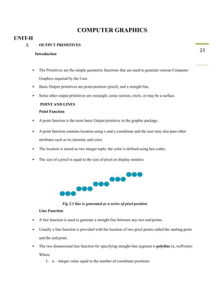
  • 1. COMPUTER GRAPHICS UNIT-II 2. OUTPUT PRIMITIVES Introduction 21 ▪ The Primitives are the simple geometric functions that are used to generate various Computer Graphics required by the User. ▪ Basic Output primitives are point-position (pixel), and a straight line. ▪ Some other output primitives are rectangle, conic section, circle, or may be a surface. POINT AND LINES Point Function ▪ A point function is the most basic Output primitive in the graphic package. ▪ A point function contains location using x and y coordinate and the user may also pass other attributes such as its intensity and color. ▪ The location is stored as two integer tuple, the color is defined using hex codes. ▪ The size of a pixel is equal to the size of pixel on display monitor. Fig 2.1 line is generated as a series of pixel position Line Function ▪ A line function is used to generate a straight line between any two end points. ▪ Usually a line function is provided with the location of two pixel points called the starting point and the end point. ▪ The two dimensional line function for specifying straight-line segment is polyline (n, wePoints) Where 1. n – integer value equal to the number of coordinate positions.
  • 2. 2. wePoints – array of input world coordinate values. ▪ This line function is used to define a set of n-1 connected straight line segments. For example The following statements generate two connected line segments with end point (50, 100) (150, 250) and (250, 100). wcPoints • x[1] = 50; wcPoints • y[1] = 100; wcPoints • x[2] = 150; wcPoints • y[2] = 250; wcPoints • x[3] = 250; wcPoints • y[1] = 100;
  • 3. 22 Algorithms for displaying straight lines are based on the line equation 1 and the calculations given in Eqs. 2 and 3. For any given x interval ∆x along a line, we can compute the corresponding y interval ∆y from Eq.2 as
  • 4. ∆y = m · ∆x 4 Similarly, we can obtain the x interval ∆x corresponding to a specified ∆y as 23 ∆x = ∆y / m 5 For lines with slope magnitudes |m| < 1, ∆x can be set proportional to a small horizontal deflection voltage, and the corresponding vertical deflection is then set proportional to ∆y as calculated from Eq-4. For lines whose slopes have magnitudes |m| > 1, ∆y can be set proportional to a small vertical deflection voltage with the corresponding horizontal deflection voltage set proportional to ∆x, calculated from Eq.5. For lines with m = 1, ∆x = ∆y and the horizontal and vertical deflections voltages are equal. In each case, a smooth line with slope m is generated between the specified endpoints. On raster system, lines are plotted with pixels, and step sizes in the horizontal and vertical directions are constrained by pixel separations. Scan conversion process for straight lines is illustrated in Fig 2.3. DDAAlgorithm The digital differential analyzer (DDA) is a scan-conversion line algorithm based on calculating either ∆y or ∆x, using Eq. 4 or Eq. 5. First consider a line with positive slope, as shown in Fig. If the slope is less than or equal to 1, sample at unit x intervals (∆x = 1) and compute successive y values as yk+1 = yk + m 6 Fig 2.4 straight line segment with five sampling positions along the x axis between x1 and x2. Subscript k takes integer values starting from 0, for the first point, and increases by 1 until the final endpoint is reached. Since m can be any real number between 0.0 and 1.0, each calculated y value must be rounded to the nearest integer corresponding to a screen pixel position in the x column. For lines with a positive slope greater than 1.0, reverse the roles of x and y. That is, we sample at unit y intervals (∆y = 1) and calculate consecutive x values as x k+1 = xk + 1/m 7
  • 5. In this case, each computed x value is rounded to the nearest pixel position along the current y scan line. 24 Equations 6 and 7 are based on the assumption that lines are to be processed from the left endpoint to the right endpoint Fig 2.2. If this processing is reversed, so that the starting endpoint is at the right, then either we have ∆x = −1 and yk+1 = yk - m 8 or (when the slope is greater than 1) we have ∆y = −1 with xk+1 = xk – 1/ m 9 Negative slopes are calculated using Eq-s 6 through 9. If the absolute value of the slope is less than 1 and the starting endpoint is at the left, we set ∆x = 1 and calculate y values with Eq-6. When the starting endpoint is at the right (for the same slope), we set ∆x = −1 and obtain y positions using Eq. 8. For a negative slope with absolute value greater than 1, we use ∆y = −1 and Eq. 9 or we use ∆y = 1 and Eq.7. Algorithm #define ROUND (a) ((int) (a+0.5)) void lineDDA (int xa, int ya, int xb, int yb) { int dx = xb - xa, dy = yb - ya, steps, k; float xIncrement, yIncrement, x = xa, y = ya; if (abs (dx) > abs (dy) steps = abs (dx) ; else steps = abs dy); xIncrement = dx / (float) steps; yIncrement = dy / (float) steps; setpixel (ROUND(x), ROUND(y) ); for(k=0;k<steps;k++) { x += xIncrement’ y += yIncrement; setpixel((Round(x),Round (y)) Algorithm Description Step 1: Accept Input as two endpoint pixel positions (xa, ya), (xb, yb) Step 2: Horizontal and vertical differences between the endpoint positions are assigned to parameters dx and dy (Calculate dx = xb-xa and dy = yb-ya). Step 3: The difference with the greater magnitude determines the value of parameter steps. Step 4: Starting with pixel position (xa, ya), determine the offset needed at each step to generate the next
  • 6. pixel position along the line path.
  • 7. Step 5: loop the following process for steps number of times 1. Use a unit of increment or decrement in the x and y direction 25 2. if xa is less than xb the values of increment in the x and y directions are 1 and m 3. if xa is greater than xb then the decrements -1 and – m are used. Example: Consider the line from (0, 0) to (4, 6) 1. xa = 0, ya = 0 and xb = 4 yb = 6 2. dx = xb - xa = 4-0 = 4 and dy = yb - ya = 6-0 = 6 3. x = 0 and y = 0 4. 4 > 6 (false) so, steps = 6 5. Calculate xIncrement = dx/steps = 4 / 6 = 0.66 and yIncrement = dy/steps = 6/6 = 1 6. Setpixel(x, y) = Setpixel(0, 0) (Starting Pixel Position) 7. Iterate the calculation for xIncrement and yIncrement for steps (6) number of times 8. Tabulation of the each iteration is given below. Resultant Diagram for the above tabulation: Fig 2.5 Pixel positions along the line path between endpoints (0, 0) and (4, 6) plotted with DDA line algorithm Advantages of DDAAlgorithm 1. It is the simplest algorithm 2. It is a is a faster method for calculating pixel positions Disadvantages of DDAAlgorithm 1. Floating point arithmetic in DDA algorithm is still time-consuming 2. End point accuracy is poor
  • 8. Bresenham’s Line Algorithm ▪ An accurate and efficient raster line-generating algorithm developed by Bresenham that uses only 26 incremental integer calculations. ▪ In addition,Bresenham’s line algorithm can be adapted to display circles and other curves. ▪ To illustrate Bresenham’s approach, we first consider the scan-conversion process for lines with positive slope less than 1.0. ▪ Pixel positions along a line path are determined by sampling at unit x intervals. Starting from the left endpoint (x0, y0) of a given line, we step to each successive column (x position) and plot the pixel whose scan-line y value is closest to the line path. Assuming we have determined that the pixel at (xk , yk ) is to be displayed, next we need to decide which pixel to plot in column xk+1. Our choices are the pixels at positions (xk + 1, yk ) and (xk + 1, yk + 1). For example, is shown in the following figure 2.4. From position (2, 3) we need to determine at next sample position is whether (3, 3) or (3, 4). We choose the point which is closer to the original line. Fig 2.6 a straight line segment is to be plotted, starting from the pixel at column 2 on scan line 3. At sampling position xk + 1, we label vertical pixel separations from the mathematical line path as dlower and dupper in Fig 2.5.
  • 9. Fig 2.7 Distance between pixel position
  • 10. The y coordinate on the mathematical line at pixel column position xk + 1 is calculated as y = m (xk+1) + b ----------------------------- 10 27 Then dlower = y - yk = m ( x k + 1 ) + b - y k A n d dupper = (yk +1) – y = yk +1 - m (xk+1) – b The difference between these two separations is dlower- dupper = 2m(xk + 1) – 2yk +2b – 1 11 A decision parameter pk for the kth step in the line algorithm can be obtained by rearranging Eq. 11 By substituting m = ∆x / ∆y we get Pk = ∆x (dlower-dupper) =2∆y.xk-2∆x.yk+c 12 The sign of pk is the same as the sign of dlower – dupper. At step k + 1, the decision parameter is evaluated from Eq. 12 as pk+1 = 2∆y · xk+1 − 2∆x · yk+1 + c Subtracting Eq. 12 from the preceding equation, we have
  • 11. pk+1 − pk = 2 ∆y(xk+1 − xk ) − 2 ∆x(yk+1 − yk ) But xk+1 = xk + 1, so that pk+1 = pk + 2 ∆y − 2 ∆x(yk+1 − yk ) 13 Where the term yk+1 − yk is either 0 or 1, depending on the sign of parameter pk . ▪ This recursive calculation of decision parameters is performed at each integer x position, starting at the left coordinate endpoint of the line. ▪ The first parameter, p0, is evaluated from Eq.12 at the starting pixel position (x0, y0) and with m evaluated as ∆y / ∆x: p0 = 2∆y −∆x 14 Bresenham’s Line-Drawing Algorithm for |m| < 1 1. Input the two line endpoints and store the left endpoint in (x0, y0) 2. Set the color for frame-buffer position (x0, y0); i.e., plot the first point. 3. Calculate the constants ∆x, ∆y, 2∆y, and 2∆y − 2∆x, and obtain the starting value for the decision parameter as p0 = 2∆y − ∆x
  • 12. 4. At each xk along the line, starting at k = 0, perform the following test. If pk < 0, the next point to plot is (xk + 1, yk ) and 28 pk+1 = pk + 2∆y 5. Otherwise, the next point to plot is (xk + 1, yk + 1) and pk+1 = pk + 2∆y − 2∆x 6. Perform step 4 ∆x − 1 times. Implementation of Bresenham Line drawing Algorithm void lineBres (int xa, int ya, int xb, int yb) { int dx = abs( xa – xb) , dy = abs (ya - yb); int p = 2 * dy – dx; int twoDy = 2 * dy, twoDyDx = 2 *(dy - dx); int x , y, xEnd; /* determine which point to use as start, which as end */ if (xa > x b ) { } else { } x = x b ; y = y b ; xEnd = xa; x = x a ; y = y a
  • 13. ; xEnd = xb; setPixel(x, y); while(x < xEnd) { else x++; if (p < 0) p+ = twoDy; { y++; p+ = twoDyDx; } setPixel(x,y); } }
  • 14. Example: Consider the line with endpoints (20, 10) to (30, 18) 29 The line has the slope m = (18 - 10)/ (30 - 20) = 8/10 = 0.8 Δx = 10 Δy = 8 The initial decision parameter has the value p0 = 2Δy - Δx = 6 and the increments for calculating successive decision parameters are 2Δy = 16 2Δy - 2 Δx = -4 We plot the initial point (x0, y0) = (20, 10) and determine successive pixel positions along the line path from the decision parameter. Tabulation: 2.8 Pixel positions along the line path between endpoints (20, 10) and (30, 18) plotted with Bresenham’s line algorithm Advantages 1. Algorithm is fast 2. Uses only integer calculations Disadvantages 1. It is meant only for basic line drawing. LOADING THE FRAME BUFFER ● After scan converting the straight line segments and other objects in the raster system, frame buffer positions must be calculated.
  • 15. ● It is done by set pixel procedure that stores intensity values for the pixels at corresponding addresses within the frame buffer array. 30 ● Scan conversion algorithms generate pixel positions at successive intervals. ● To calculate frame-buffer addresses, incremental methods are used. Figure 2.10 Circle with Center Coordinate (xc, yc) and Radius r
  • 16. The distance relationship is expressed by the Pythagorean Theorem in Cartesian coordinates as follows (x – xc)2 +(y – yc)2 = r2 31 y values at each position is calculated as and the x axis steps from xc – r to xc + r. This method is not a best method for generating a circle. Problems (1) It involves considerable computation at each step. (2) The spacing between each plotted pixel position is not uniform. Solutions (1) The spacing can be adjusted by interchanging x and y whenever the absolute value of the slope of the circle is greater than 1. ● It increases the computation and processing of the algorithm. (2) Another way to adjust the unequal spacing is to calculate points along the circular boundary using polar coordinates r and θ. ● The circle equation in parametric polar form yields the following pair of equations: x = xc+r cosθ y = yc+r sinθ Where θ is a fixed angular step size. By using the above equation, a circle is plotted with equally spaced points along the circumference. Symmetry of a circle •By considering the symmetry of a circle, computations can be reduced. •The shape of the circle is similar in all the four quadrants.
  • 17. Figure 2.11: Symmetry of a circle ● There is symmetry between octants (shown in figure 2.11).
  • 18. ● Circle sections in adjacent octants within one quadrant are symmetric with respect to the 45° line dividing the two octants. 32 Advantage ● We can generate all pixel positions around a circle by calculating only the points within the sector from x=0 to x=y. MIDPOINT CIRCLE ALOGITHM Figure 2.12 Mid Point between Candidate Pixels
  • 19. 33
  • 20. ● The start position (0, r) with the value (0, 2r). ● Successive values are obtained by adding 2 to the previous value of 2x, and subtracting 2 from 34 the previous value of 2y.
  • 21. 35
  • 22. ATTRIBUTES OF OUTPUT PRIMITIVES Any parameter that affects the way a primitive is to be displayed is referred to as an 36 attribute parameter. Attribute parameters are color, size etc. It is used to determine the fundamental characteristics of a primitive. TYPES OF ATTRIBUTES 1. Line Attributes 2. Curve Attributes 3. Color and Grayscale Levels 4. Area Fill Attributes 5. Character Attributes 6. Bundled Attributes Line Attributes Basic attributes of a straight line segment are 1. Line Type 2. Line Width 3. Pen and Brush Options 4. Line Color Line type Line type attribute includes solid lines, dashed lines and dotted lines. To set line type attributes in a PHIGS application program, a user invokes the function setLinetype (lt) where parameter lt is assigned a positive integer value of 1, 2, 3 or 4 to generate lines that are solid, dashed, dash dotted respectively. Other values for line type parameter it could be used to display variations in dot-dash patterns. Line width Implementation of line width option depends on the capabilities of the output device to set the line width attributes. To set the line-width attributes using the following command setLinewidthScaleFactor (lw) ▪ Line width parameter lw is assigned a positive number to indicate the relative width of line to be displayed. ▪ A value of 1 specifies a standard width line. ▪ To set lw to a value of 0.5 to plot a line whose width is half that of the standard line.
  • 23. ▪ Values greater than 1 produce lines thicker than the standard.
  • 24. Line Cap ▪ To adjust the shape of the line ends to give them a better appearance by adding line cap (Fig: 2.8). 37 ▪ There are three types of line cap. They are 1. Butt cap 2. Round cap 3. Projecting square cap Fig 2.14 Types of Line Joining Miter join It is accomplished by extending the outer boundaries of each of the two lines until they meet.
  • 25. Round join It is produced by capping the connection between the two segments with a circular boundary 38 whose diameter is equal to the width. Bevel join It is generated by displaying the line segment with but caps and filling in triangular gap where the segments meet. Pen and Brush Options ▪ In some graphics packages, lines can also be displayed using selected pen or brush options. ▪ Options in this category include shape, size, and pattern. Some possible pen or brush shapes are given in following figure 2.10. Fig 2.15 Various Pen and Brush Shapes Line color ▪ A poly line routine displays a line in the current color by setting this color value in the frame buffer at pixel locations along the line path using the set pixel procedure. ▪ To set the line color value in PHlGS with the function setPolylineColourIndex (lc) Non negative integer values, corresponding to allowed color choices, are assigned to the line color parameter lc. Example: Various line attribute commands in an applications program is given by the following sequence of statements Area Fill Attributes
  • 27. r I i n d e x ( 6 ) ; p o l y l i n e ( n 2 , w c p o i n t s 2 ) ; Options for filling a defined region include a choice between a solid color and a pattern fill and choices for particular colors and patterns. These fill options can be applied to polygon regions or to areas defined with curved boundaries depending on the capabilities of available package.
  • 28. The areas can be displayed using various brush styles, colors and transparency parameters. Fill Styles 39 Areas are displayed with three basic fill styles, are shown in Fig: 2.11. 1. Hollow with a color border 2. Filled with a solid color 3. Filled with a specified pattern or design. Fig 2.16 Polygon Fill styles A basic fill style is selected in a PHIGS program with the function setInteriorStyle (fs) ▪ Values for the fill-style parameter fs include hollow, solid, and pattern. ▪ Another value for fill style is hatch, which is used to fill an area with selected hatching patterns such as parallel lines or crossed lines. ▪ The color for a solid interior or for a hollow area outline is chosen with where fill color parameter fc is set to the desired color code setInteriorColourIndex (fc) where fill-color parameter fc is set to the desired color code. Some other fill options are used to specify the edge type, edge width and edge color of a region. Pattern Fill To select fill patterns with the following function setInteriorStyleIndex (pi) Where pattern index parameter pi specifies a table position For example, the following set of statements would fill the area defined in the fillArea command with the second pattern type stored in the pattern table:
  • 30. function 40 For fill style pattern, table entries can be created on individual output devices with the following setPatternRepresentation (ws,pi,nx,ny,cp) Parameter pi sets the pattern index number for workstation code ws, and cp is a two dimensional array of color codes with nx columns and ny rows. For example the following function could be used to set the first entry in the pattern table for workstation 1. setPatternRepresentation (1,1,2,2,cp); When color array cp is to be applied to fill a region, we need to specify the size of an array with the following function setPatternSize( dx,dy) Where parameters dx and dy give the coordinate width and height of the array mapping. Then a reference position for starting a pattern fill is assigned with the following statement; setPatternReferencePoint (position); Where parameter position is a pointer to coordinates (xp,yp) that fix the lower left corner of the rectangular pattern. Tiling: The process of filling an area with a rectangular pattern is called tiling and it is also referred to as tiling patterns. Soft Fill: Soft fill or tint fill algorithms are applied to repaint areas so that the fill color is combined with background color. An example of this type of fill is linear soft fill algorithm repaints an area by merging a fore ground color F with a single background color B, Where F is not equal B. Character Attributes ▪ The appearance of displayed character is controlled by attributes such as font, size, color and
  • 32. ▪ Attributes can be set both for entire character strings (text) and for individual characters defined as marker symbols. 41 Text Attributes ▪ The choice of font or type face is set of characters with a particular design style as courier, Helvetica, times roman, and various symbol groups. ▪ The characters in a selected font also are displayed with styles (solid, dotted, double) in bold face in italics and in outline or shadow styles. A particular font and associated style is selected in a PHIGS program by setting an integer code for the text font parameter tf in the function setTextFont (tf) Control of text color (or intensity) is managed from an application program with setTextColourIndex (tc) Where text color parameter tc specifies an allowable color code. We can adjust text size by scaling the overall dimensions of characters or by scaling only the character width. Character size is specified by points, where 1 point is 0.013837 inch. Point measurements specify the size of the body of a character. The distance between the bottom-line and the top line of the character body is same for all characters in particular size and typeface, but width of the body may vary. Proportionally spaced fonts assign a smaller body width to narrow characters such as i, j, l and f compared to broad characters such as W or M. Character height is defined as the distance between the base line and cap line of characters. Text size can be adjusted without changing the width to height ratio of characters with setCharacterHeight (ch) Parameter ch is assigned a real value greater than 0 to set the coordinate height of capital letters. The width of text can be set with function. setCharacterExpansionFactor (cw) Where the character width parameter cw is set to a positive real value that scales the body width
  • 34. 42 Spacing between characters is controlled separately with setCharacterSpacing (cs) vector Where the character-spacing parameter cs can he assigned any real value. The orientation for a displayed character string is set according to the direction of the character up setCharacterUpVector (upvect) Parameter upvect in this function is assigned two values that specify the x and y vector components. Text is displayed so that the orientation of characters from base line to cap line is in the direction of the up vector. For example, upvect = (1, 1) is displayed the text in 450 as shown in the following figure.
  • 35. To arrange character strings vertically or horizontally setTextPath (tp) 43 tp can be assigned the value: right, left, up, or down Another attribute for character strings is alignment. This attribute specifies how text is to be positioned with respect to the start coordinates. Alignment attributes are set with SetTextAlignment (h,v) Where parameters h and v control horizontal and vertical alignment. GNIRTS STRING Horizontal alignment is set by assigning h a value of left, center, or right. Vertical alignment is set by assigning v a value of top, cap, half, base or bottom. A precision specification for text display is given with SetTextPrecision (tpr) tpr is assigned one of values string, char or stroke. Marker Attributes Marker symbol is a single character that can he displayed in different colors and in different sizes. To select a particular character to be the marker symbol with setMarkerType (mt) Where marker type parameter mt is set to an integer code Typical codes for marker type are the integers 1 through 5, specifying, respectively, a dot (.) a vertical cross (+), an asterisk (*), a circle (o), and a diagonal cross (X). To set the marker size with setMarkerSizeScaleFactor (ms) With parameter marker size ms assigned a positive number. This scaling parameter is applied to the nominal size for the particular marker symbol. Values greater than 1 increase the marker size and values less than one reduce the marker size.
  • 36. Marker color is specified with SetPolymarkerColourIndex (mc) 44 Selected color code parameter mc is stored in the current attribute list and used to display subsequently specified marker primitives Bundled Attributes A single attribute that specifies exactly how a primitive is to be displayed with that attribute setting. These specifications are called individual or unbundled attributes. A particular set of attributes values for a primitive on each output device is chosen by specifying appropriate table index. Attributes specified in this manner are called bundled attributes. The table for each primitive that defines groups of attribute values to be used on particular output devices is called a bundle table. The choice between a bundled or an unbundled specification is made by setting a switch called the aspect source flag for each of these attributes setIndividualASF( attributeptr, flagptr) Where parameter attributerptr points to a list of attributes and parameter flagptr points to the corresponding list of aspect source flags. Each aspect source flag can be assigned a value of individual or bundled. Bundled line Attributes Entries in the bundle table for line attributes on a specified workstation are set with the function setPolylineRepresentation (ws, li, lt, lw, lc) Parameter ws is the workstation identifier and line index parameter li defines the bundle table position. Parameter lt, lw, tc are then bundled and assigned values to set the line type, line width, and line color specifications for designated table index. Example setPolylineRepresentation (1, 3, 2, 0.5, 1) setPolylineRepresentation (4, 3, 1, 1, 7) A poly line that is assigned a table index value of 3 would be displayed using dashed lines at half thickness in a blue color on work station 1; while on workstation 4, this same index generates solid, standard-sized white lines.
  • 37. Once the bundled tables have been set up, a group of bundled line attributes is chosen for each workstation by specifying table index value;
  • 38. Bundled Area fills Attributes setPolylineIndex (li); 45 Table entries for bundled area-fill attributes are set with setInteriorRepresentation (ws, fi, fs, pi, fc) Which defines the attributes list corresponding to fill index fi on workstation ws. ● Parameter fs, pi and fc are assigned values for the fill style, pattern index and fill color respectively. ● A particular attribute bundle is selected from the table with the function setInteriorIndex (fi); Bundled Text Attributes Table entries for bundled text attributes are set with setTextRepresentation (ws, ti, tf, tp, te, ts, tc) Bundles values for text font, precision,expansion factor, size and color in a table position for work station ws that is specified by value assigned to text index parameter ti. A particular text index value is chosen with the function setTextIndex (ti); Bundled Marker Attributes Table entries for bundled marker attributes are set with setPolymarkerRepresentation (ws, mi, mt, ms, mc) That defines marker type, marker scale factor, marker color for index mi on workstation ws. Bundle table selections are made with the function setPolymarkerIndex (mi); COLOUR AND GRAYSCALE LEVELS ● Colour options are numerically coded with values ranging from 0 through the positive integers. These color codes are converted to intensity level settings for the electron beams in CRT monitors. ● Color Tables ● Color information can be stored in the frame buffer in two ways : o The colour codes can be directly put in the frame buffer (or) o Colour codes can be maintained in a separate table and pixel values can be used as an index into this table.
  • 39. 46 Figure.2.17: Colour look-up table Advantages of storing colour codes in lookup table (1) Colour table can provide a reasonable number of simultaneous colours without requiring large frame buffers. (2) Table entries can be changed at anytime, and allows the user to experiment easily with different color combinations in a design, scene or graph without changing the attribute settings for the graphics data structure. (3) Visualization applications can store values for some physical quantity such as energy in the frame buffer. (4) Use lookup table to get various color encodings without changing the pixel values. (5) In visualization and image processing applications, color tables are used for setting color thresholds so that all pixel values above or below a specified threshold can be set the same colour. Grayscale ● With monitors that have no color capability, color functions can be used in an application program to set the shades of gray, or grayscale for the displayed primitives. ● Numeric values from 0 to 1, can be used to specify grayscale levels, which are converted to appropriate binary codes for storage in the raster. ● The table given below shows the specification for intensity codes for a four level grayscale
  • 41. ● Intensity is calculated based on the colour index as follows: Intensity = 0.5 [min (r,g,b) + max (r,g,b)] INQUIRY FUNCTION ● Inquiry functions are used to retrieve the current settings of attributes and other parameters such as workstation types and status from the system lists. ● By using inquiry function, current values of any specified parameter can be saved and then they can be reused later or they can be used to check the current state of the system if any error encounters. ● Current attribute values are checked by specifying the name of the attribute in the inquiry function as follows inquirePolylineIndex (last li) To copy the current values of attributes inquireInteriorColorIndex (last_fc) ● The above function the current values of line index and fill color into parameters last last li and lastfc.