Microgreens have many beneficial properties such as their unique colors, flavor profiles, and textures while also having higher concentrations of secondary metabolites than more mature plants which can help fill existing nutritional gaps in human diets. The influence of both light quality and quantity on microgreen production (yield and secondary metabolites) is an ongoing research endeavor. The objective of this review paper was therefore to investigate the links between the type and amount of light with Brassicaceae microgreen Dry Weight (DW), Anthocyanin, and Carotenoid accumulation by using multilinear regressions.

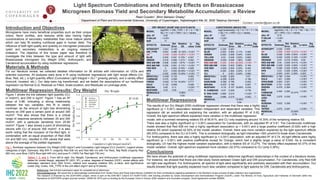
1. Light Spectrum Combinations and Intensity Effects on Brassicaceae
Microgreen Biomass Yield and Secondary Metabolite Accumulation: a Review
Introduction and Objectives
Microgreens have many beneficial properties such as their unique
colors, flavor profiles, and textures while also having higher
concentrations of secondary metabolites than more mature plants
which can help fill existing nutritional gaps in human diets. The
influence of both light quality and quantity on microgreen production
(yield and secondary metabolites) is an ongoing research
endeavor. The objective of this review paper was therefore to
investigate the links between the type and amount of light with
Brassicaceae microgreen Dry Weight (DW), Anthocyanin, and
Carotenoid accumulation by using multilinear regressions.
Reed Cowden1, Bhim Bahadur Ghaley1
1Department of Plant and Environmental Sciences, University of Copenhagen, Højbakkegård Alle 30, 2630 Taastrup Denmark
Contact: cowden@plen.ku.dk
References: See full-text submission paper for complete list of references.
Acknowledgements: We would like to acknowledge contributions from Teodor Rusu and Paula Ioana Moraru (USAMV) for their contributions regarding assistance in the literature review process of data collection and organization.
The research is financed by the GOHYDRO project, which is part of the ERA-NET Cofund ICT-AGRI-FOOD, with funding provided by Green Development and Demonstration Program (GUDP), under The Ministry of Food, Agriculture and Fisheries of Denmark within the
framework of GOHYDRO project (journal number: 34009-20-1815) and co-funding by the European Union’s Horizon 2020 research and innovation program, Grant Agreement number 862665.
For our literature review, we collected detailed information on 36 articles with information on LEDs and
selected outcomes. All analyses were done in R using multilinear regressions with light recipe effects (UV,
Blue, Red, etc.), a light quantity effect (Cumulative Light Integral = DLI * growing period), and a variety effect
(broccoli, mustard, etc.). Our data were log transformed, and we tested the assumptions of our multilinear
regression via Normal Q-Q, Residual vs Fitted, Scale-location, and Residuals vs Leverage plots.
Materials & Methods
Multilinear Regression Results: Dry Weight
Conclusions
We have shown the potential of using multilinear regressions to determine significant relationships in the context of a literature review.
For instance, we showed that there are inter-study trends between Green light and DW accumulation. For Carotenoids, only Red 638
nm light was significant. For Anthocyanins, all spectra of light were significantly and positively associated with their accumulation. Our
results showed that light quantity explained much less variation compared to light spectra for DW, Carotenoids and Anthocyanins.
There was also a highly significant (p < 0.001) association for Carotenoids, with an adjusted R2 of 0.81. The Carotenoids multilinear
model showed that Red 638 nm had a highly significant association (p < 0.001) and a large positive coefficient (0.025) with a high
relative SS which explained 42.55% of the model variation. Overall, there was more variation explained by the light spectrum effects
(65.33%) compared to the CLI of 0.04%. This is consistent biologically, as light intensities >300 µmol/m2/s break down Carotenoids.
For Anthocyanins, there was also a highly significant (p < 0.001) association, with an adjusted R2 of 0.74. All light effects were highly
significant (p < 0.001) with positive coefficients except for Orange, which had a slightly larger p-value of 0.040. As is consistent
biologically, UV had the highest model variation explanation, with a relative SS of 13.27%. The Variety effect explained 43.37% of the
model variation. Overall, light spectrum explained more variation (32.57%) compared to CLI (only 0.36%).
The results of our Dry Weight (DW) multilinear regression showed that there was a highly
significant (p < 0.001) association between independent and dependent variables. This
regression did an excellent job explaining the variation, with an adjusted R2 of 0.92.
Overall, the light spectrum effects explained more variation in the multilinear regression
Tables 1, 2, and 3. From left to right: Dry Weight, Carotenoid, and Anthocyanin multilinear regression
tables for model design, adjusted R2 (ADJ. R2), p-value, degrees of freedom (DOF), model effects with
estimates, standard error (Std. Error), relative sum squares (relative SS), p-value, and significance
codes (Sig. Code). DW_TYPE is the unit effect (kg/m2 and g/10 plants).
Multilinear Regressions
DRY WEIGHT (KG/M2
AND G/10 PLANTS)
MODEL
log(DW) = DW_TYPE + B + G + Rb +
Ra + Fr + UV + HPS + CLI + Variety
ADJ. R2
0.92
P-VALUE < 0.001
DOF 77
EFFECTS Estimate
Std.
Error
Relative
SS
p-
value
Sig.
Code
INTERCEPT -3.941 0.145
DW_TYPE 0.623 0.086 61.05% < 0.001 ***
UV -0.246 0.029 15.20% *< 0.001 ***
BLUE 0.003 0.001 0.15% * 0.047 *
GREEN 0.018 0.006 1.21% * 0.002 **
RED 638 NM 0.008 0.002 1.87% * < 0.001 ***
RED 660 NM 0.005 0.001 2.11% * < 0.001 ***
FAR RED 0 0.002 9.78% * 0.929
HPS 0.01 0.002 20.49% *< 0.001 ***
CLI 0.002 0.000 15.30% *< 0.001 ***
BROCCOLI -0.429 0.134 0.002 **
CABBAGE 0.072 0.059 0.223
CRESS -0.042 0.116 16.02% * 0.717
KALE 0.132 0.059 0.028 *
MIZUNA 0.65 0.11 < 0.001 ***
MUSTARD 0.02 0.05 0.711
RESIDUALS 6.96%
R2
0.93
CAROTENOIDS (MG/KG FW)
MODEL
log(Carotenoids) = B + G + O + Y + Rb
+ Ra + Fr + HPS + CLI + Variety
ADJ. R2
0.81
P-VALUE < 0.001
DOF 77
EFFECTS Estimate
Std.
Error
Relative
SS
p-value
Sig.
Code
INTERCEPT 4.238 0.281
BLUE 0.003 0.004 2.11% 0.482
GREEN 0.002 0.008 5.45% 0.804
YELLOW 0.02 0.046 3.63% 0.665
ORANGE -0.024 0.046 1.90% 0.599
RED 638 NM 0.025 0.004 42.55% < 0.001 ***
RED 660 NM 0.004 0.003 8.96% 0.164
FAR RED -0.003 0.004 0.53% 0.493
HPS 0.005 0.004 0.20% 0.147
CLI 0 0.001 0.04% 0.983
BROCCOLI -0.482 0.263 0.07 .
KALE -0.299 0.209 0.156
KOHLRABI -0.382 0.195 0.053 .
MIZUNA -0.537 0.195 0.007 **
MUSTARD -0.19 0.157 18.66% 0.232
R. CABBAGE -0.07 0.209 0.738
R. PAK CHOI 0.869 0.215 < 0.001 ***
TATSOI 0.696 0.215 0.002 **
RESIDUAL 15.98%
R2
0.84
ANTHOCYANINS (MG/KG FW)
MODEL
log(Anth) = B + G + O + Rb + Ra + Fr +
UV + HPS + CLI + Variety
ADJ. R2
0.74
P-VALUE < 0.001
DOF 198
EFFECTS Estimate
Std.
Error
Relative
SS
p-value
Sig.
Code
INTERCEPT 0.026 0.505
UV 0.058 0.005 13.27% < 0.001 ***
BLUE 0.038 0.005 0.95% < 0.001 ***
GREEN 0.035 0.005 0.18% < 0.001 ***
ORANGE 0.03 0.015 0.05% 0.04 *
RED 638 NM 0.04 0.005 9.41% < 0.001 ***
RED 660 NM 0.029 0.005 4.06% < 0.001 ***
FAR RED 0.036 0.005 0.06% < 0.001 ***
HPS 0.03 0.005 4.59% < 0.001 ***
CLI 0.003 0.001 0.36% 0.003 **
BROCCOLI 2.166 0.344
43.37%
< 0.001 ***
KALE 1.421 0.269 < 0.001 ***
KOHLRABI 2.943 0.321 < 0.001 ***
MUSTARD 2.741 0.235 < 0.001 ***
RADISH 4.078 0.364 < 0.001 ***
RED
CABBAGE
2.494 0.284 < 0.001 ***
RED PAK
CHOI
3.275 0.235 < 0.001 ***
RED
RUSSIAN
KALE
3.633 0.359 < 0.001 ***
TATSOI 3.072 0.247 < 0.001 ***
RESIDUAL 23.69%
R2
0.76
model, with a summed remaining relative SS of 50.81%, and CLI only explaining around 15.30% of the remaining relative SS.
Figure 1 shows the link between light quantity (CLI
in mol/m2), and DW in kg/m2. Figure 1 has an R2
value of 0.88, indicating a strong relationship
between the two variables; this fit is clearly
nonlinear, as the amount of light has diminishing
returns on DW past a certain point at around 300
mol/m2. This also shows that there is a critical
range of response sensitivity between 25 and 200
mol/m2, with a particular sensitivity from 25-60
mol/m2. Figure 1 also shows a point of diminishing
returns with CLI of around 300 mol/m2. It is also
worth noting that the inclusion of Far-Red light, in
combination with an equal proportion of Red (638
nm and 660 nm), resulted in DW values that were
above the average of the plotted regression.
Fig 1. Nonlinear regression between Dry Weight (DW) (kg/m2) and Cumulative Light Integral (CLI) (mol/m2). Legend shows
categories of light: Darkness, Maj R/R Fr (majority Red 638 nm and Red 660 nm with Far Red), Maj Redb (majority Red
660 nm), pure Blue (100% Blue light 445 nm), and pure Fr (100% Far Red light 730 nm).