SlideShare a Scribd company logo
1 of 131
Download to read offline
ECE 285
Image and video restoration
Chapter V – Bayesian methods
Charles Deledalle
March 21, 2019
1
Multiview restoration – Motivation
• Given m corrupted images y1
, . . . , ym
of a same clean image x
• What is the best approach to retrieve x?
2
Multiview restoration – Sample mean
Average, a.k.a., sample mean estimator
ˆx =
1
m
m
k=1
yk
Why does it performs denoising?
3
Multiview restoration – Sample mean
Average, a.k.a., sample mean estimator
• Assume yk
are iid (independent and identically distributed), then
E[ˆx] = E
1
m
m
k=1
yk
=
1
m
m
k=1
E yk
= E yk
⇒ If E yk
= x, the sample-mean is unbiased.
• and Var[ˆx] = Var
1
m
m
k=1
yk
=
1
m2
m
k=1
Var yk
=
1
m2
m
k=1
σ2
=
σ2
m
⇒ Sample-mean reduces the fluctuations by
√
m.
4
Multiview restoration – Sample mean
ˆx =
1
m
m
k=1
yk
(Weak) Law of large numbers
plim
m→∞
ˆx = x ⇔ ∀ε > 0, lim
m→∞
P[||ˆx − x||2 ε] = 0
The sample mean ˆx is said to be a consistent estimator of x.
As the number of views increase,
the restoration improves with high probability.
5
Multiview restoration – Sample mean
(a) yk
(Gaussian noise) (b) m=9 (SNR ×3) (c) m=81 (SNR ×9)
≈
(d) x
SNR =
E[ˆx]
Var[ˆx]
=
√
mx
σ
−−−−−−−→
m→∞
∞
But what if the assumptions are violated?
6
Multiview restoration – Sample mean
(a) yk
(Impulse noise) (b) m = 9 (c) m = 81
≈
(e) ˆx
For impulse noise E[yk
] = x
If the assumptions are violated
1 May not converge towards x (biased estimation).
2 May not even converge.
7
Multiview restoration – Sample mean
(a) yk
(Cauchy noise) (b) m = 9 (c) m = 81
≈
(e) ˆx
For Cauchy noise E[yk
] and Var[yk
] do not exist!
If the assumptions are violated
1 May not converge towards x (biased estimation).
2 May not even converge.
8
Multiview restoration – Sample mean
(a) yk
(Cauchy noise) (b) m = 9 (c) m = 81
≈
(e) ˆx
For Cauchy noise E[yk
] and Var[yk
] do not exist!
If the assumptions are violated
1 May not converge towards x (biased estimation).
2 May not even converge.
Even though: the convergence can be too slow.
8
Multiview restoration – Alternatives
Possible alternatives:
Samples yk
= 4, 10, 3, 6, 2, 3, 2, 2, 4
• Sample mean (average)
4+10+3+6+2+3+2+2+4
9
= {4}
• Sample median (middle one)
2, 2, 2, 3, 3, 4, 4, 6, 10
• Sample mode (most frequent ones)
3×2, 2×3, 2×4, 1×6, 1×10
Estimator
Random variable Y
• Mean (expectation):
E[Y ] =
+∞
−∞
yp(y; x) dy
• Median:
m
−∞
p(y; x) dy =
∞
m
p(y; x) dy =
1
2
• Mode (distribution peaks):
argmax
y
p(y; x)
Quantity being estimated
Which one should I pick?
9
Multiview restoration – Alternatives
0 2 4 6 8 10
0
0.1
0.2
0.3
0.4
0.5
(a) Gaussian law
0 2 4 6 8 10
0
0.1
0.2
0.3
0.4
0.5
0.6
(b) Laplace law
0 2 4 6 8 10
0
0.05
0.1
0.15
0.2
0.25
0.3
0.35
0.4
(c) Cauchy law
0 2 4 6 8 10
0
0.05
0.1
0.15
0.2
0.25
(d) Poisson law
0 2 4 6 8 10
0
0.05
0.1
0.15
0.2
(e) Gamma law
0 2 4 6 8 10
0
0.05
0.1
0.15
0.2
0.25
0.3
0.35
0.4
(f) Impulse law
• Mean/mode/median do not necessarily correspond to the unknown x,
• Often, function of x through a link function, ex: x = g(E[y]),
• Should take into account such a link between the images yk
and x.
10
Multiview restoration – Method of moments
Method of moments (Karl Pearson, 1894)
Assume



• yk
are iid,
• x = g(E[yk
]), and
• Var[yk
] is finite.
1. Consistently estimate µ = E[yk
] by sample mean
ˆµ = ¯y =
1
m
m
k=1
yk
2. Next estimate x as
ˆx = g(ˆµ)
11
Multiview restoration – Method of moments
Properties of method of moments
• Easy to compute if we know g.
• Unbiased if g is linear.
• When g is sufficiently regular, asymptotically unbiased:
lim
m→∞
E[ˆx] = x
. . . and consistent:
plim
m→∞
ˆx = x .
• But:
• Biased for small m, since: E[g(ˆµ)] = g(E[ˆµ]),
• Often inefficient: slow convergence.
12
Multiview restoration – Method of moments
Example (Impulse noise (1/3))
• Consider y and x defined in [0, L − 1] such as
p(y ; x) =
1 − P + P/L if y = x
P/L otherwise
0 5 10 15
0
0.2
0.4
0.6
0.8
1
13
Multiview restoration – Method of moments
Example (Impulse noise (2/3))
• We have
E[y] =
L−1
y=0
yp(y; x)
= x(1 − P + P/L) + P/L
y=x
y
= x(1 − P + P/L) + P/L
L−1
y=0
y
= 1
2
(L−1)L
−x
= x(1 − P) +
1
2
P(L − 1)
• Hence E[y] = h(x) with
h(x) = x(1 − P) +
1
2
P(L − 1)
14
Multiview restoration – Method of moments
Example (Impulse noise (3/3))
• As E[y] = h(x) with
h(x) = x(1 − P) +
1
2
P(L − 1)
• If P = 1, h is invertible, and for g = h−1
, we have
x = g(E[y]) with g(µ) =
µ − 1
2
P(L − 1)
1 − P
• The moment estimator is thus
ˆx = g(¯y) =
1
m
m
k=1 yk
− 1
2
P(L − 1)
1 − P
i.e., an affine correction of the sample mean.
15
Multiview restoration – Method of moments – Results
(a) yk
(Impulse noise)
SamplemeanM.ofmom.
(b) m = 9 (c) m = 81 (d) m = 243
• Much better than the sample mean
16
Multiview restoration – Method of moments – Results
(a) yk
(Impulse noise)
SamplemeanM.ofmom.Samplemode
(b) m = 9 (c) m = 81 (d) m = 243
• Much better than the sample mean
• Clearly not as efficient as the sample mode Why?
16
Mean square error
Mean square error - Risk
Define optimality
• Choose a loss-function: (x, ˆx) such that
• (x, x) = 0
• (x, ˆx) > 0: measure the proximity
• Write: ˆx = ˆx(y1
, . . . , ym
) with ˆx : Rn
× . . . × Rn
m times
→ Rn
• Define the risk or expected loss as
R(x, ˆx) = . . . (x, ˆx(y1
, . . . , ym
)) p(y1
, . . . , ym
; x) dy1
. . . dym
or in short E[ (x, ˆx)]
17
Mean square error – Definition
Mean square error
• The choice of the loss depends on the application context.
• Most common choice for linear regression problems:
square error (or 2-loss)
(x, ˆx) = ||x − ˆx||2
2 =
n
i=1
(xi − ˆxi)2
• The expected risk is thus called Mean Square Error (MSE)
R(x, ˆx) = MSE(x, ˆx) = E||x − ˆx||2
2
18
Mean square error - Bias and Variance
Bias-variance decomposition
MSE(x, ˆx) =
n
i=1
(xi − E[ˆxi])2
+
n
i=1
Var[ˆxi]
= ||x − E[ˆx]||2
Bias2
+ tr Var[ˆx]
Variance
Minimizing the MSE ≡ Minimizing bias2
and variance
19
Mean square error – Bias and Variance
Local decomposition: bias and variance are often structure dependent
• Local map of bias: bi = |xi − E[ˆx]i| Bias2
= b2
i
• Local map of variance: vi = Var[ˆxi] Variance = vi
RAdiff.
Avg. 5.14 Avg. 11.27 Avg. 12.38
TAdiff.
(a) Result ˆx (b) Bias
Avg. 7.47
(c) Standard deviation
Avg. 6.62
(d) Root MSE
Avg. 9.98
• residual noise ≡ high estimation variance
• over-smoothing/blur ≡ bias
20
Mean square error – Bias and Variance
MSE(x, ˆx) = ||x − E[ˆx]||2
Bias2
+ tr Var[ˆx]
Variance
In general, the minimum MSE estimator has
non-zero bias and non-zero variance
Figure 1 – Smoothing more ⇒ increasing bias while reducing variance
21
Mean square error – Optimal estimation
Optimize for a class of estimators
• Choose the optimal estimator as the one minimizing the expected loss
ˆx = argmin
ˆx∈C
{R(x, ˆx) = E[ (x, ˆx)]}
for C a class of estimators.
• Without this restriction, solutions can be unrealizable,
ex: trivial solution ˆx(y1
, . . . , ym
) = x
i.e., the solution would depend on the unknown.
22
Mean square error – Optimal estimation
Example (Amplified sample mean (1/3))
• Assume yk
iid with E[yk
] = x and Var[yk
] = σ2
Idn.
• Consider the optimal estimator with respect to the MSE
ˆx = argmin
ˆx∈C
MSE(x, ˆx) = E||x − ˆx||2
2
• And the class of functions that amplify the sample mean
C =



ˆx : Rn
× . . . × Rn
m times
→ Rn
; ∃α ∈ R, ˆx(y1
, . . . , ym
) =
α
m
m
k=1
yk



• Finding ˆx leads to find α that minimizes the MSE.
23
Mean square error – Optimal estimation
ˆx(y1
, . . . , ym
) =
α
m
m
k=1
yk
Example (Amplified sample mean (2/3))
• Study the first order derivative
∂MSE(x, ˆx)
∂α
=
∂||x − E[ˆx(y)]||2
2
∂α
+
∂ tr Var [ˆx(y)]
∂α
=
∂||x − αx||2
2
∂α
+
∂α2
tr Var [y] /m
∂α
= ||x||2 ∂(1 − α)2
∂α
+
nσ2
m
∂α2
∂α
= −2||x||2
(1 − α) +
2n
m
σ2
α
• Moreover, the second order derivative is constant and positive
∂2
MSE
∂α2
= 2||x||2
+
2n
m
σ2
24
Mean square error – Optimal estimation
Example (Amplified sample mean (3/3))
• Then the MSE is a quadratic function and its minimum is given for
∂MSE
∂α
= 0 ⇔ −2||x||2
(1 − α) +
2n
m
σ2
α = 0
⇔ α =
||x||2
||x||2 + nσ2
m
Define: SNR2
=
||x||2
2
nσ2
α = SNR2
SNR2+1/m
:
• large SNR, yk
has good quality, average: ˆx = ¯y,
• low SNR, x drawn in the noise: ˆx = 0 is safer.
This is not realizable since it depends on the unknown x.
We need an alternative to direct MSE minimization.
25
Unbiased estimators
Unbiased estimators – Minimum Variance Unbiased Estimator
• In the previous example
∂MSE(x, ˆx)
∂α
=
∂Bias2
∂α
+
∂Variance
∂α
where
∂Bias2
∂α
= −2||x||2
(1 − α) and
∂Variance
∂α
=
2n
m
σ2
α
• The dependency on ||x||2
arises from the bias term,
• This occurs in many situations.
Constrain the estimator to be unbiased.
Find the estimator that produces the minimum variance.
This will provides the minimum MSE among all unbiased estimators.
26
Unbiased estimators – Minimum Variance Unbiased Estimator
Minimum Variance Unbiased Estimator (MVUE)
An estimator ˆx ∈ C is the MVUE for the class of estimators C if
(∀x, Eˆx = x)
unbiasedness
and ∀˜x ∈ C, (∀x, E˜x = x) ⇒ (∀x, tr Var[ˆx ] tr Var[˜x])
minimum variance
Example (Back to the amplified sample mean)
• An unbiased estimator that amplifies the sample mean should satisfy
Bias2
= ||x − E
α
m
m
k=1
yk
||2
= (1 − α)2
||x||2
= 0 ⇒ α = 1
• Then the sample mean is the only unbiased estimator of this class.
• It is the MVUE of this class.
27
Unbiased estimators – Minimum Variance Unbiased Estimator
Variance of 3 unbiased estimators E[ˆx1
]=E[ˆx2
]=E[ˆx3
]=x as a function of x.
Quiz: which one is the MVUE on the left? on the right?
The MVUE does not always exist.
If it does exist, how to find it?
28
Unbiased estimators – Cram´er-Rao bound
Cram´er-Rao lower bound (≈ 1945)
• Provided the bound exists, any realizable unbiased estimator satisfies
Var[ˆx] I−1
where Ii,j = E
∂2
− log p(y1
, . . . , ym
; x)
∂xi∂xj x
• Var[ˆx] I−1
means Var[ˆx] − I−1
is symmetric positive definite,
• y1
, . . . , ym
→ p(y1
, . . . , ym
; x) is the law of the observations,
• x → p(y1
, . . . , ym
; x) is the likelihood of the unknown,
• I the Fisher information matrix: expected Hessian of the log-likelihood,
• I measures the organization/entropy/simplicity of the problem,
• Ex: small noise → likelihood peaky → large Hessian → small bound.
29
Unbiased estimators – Cram´er-Rao bound
Consequence: Var[ˆx] = I−1
⇒ ˆx is the MVUE
If you find an unbiased estimator that reaches the Cram´er-Rao bound,
then it is the MVUE.
The MVUE may not reach the Cram´er-Rao bound,
in this case, no estimator reaches the bound.
30
Unbiased estimators – Efficiency
Efficiency
• The ratio 0
tr I−1
tr Var[ˆx]
1 is called efficiency of the estimator,
• Measures by how much the estimator is close to the Cram´er-Rao bound,
• An unbiased estimator with efficiency 100% is said to be efficient,
• If an efficient estimator exists, it is the MVUE,
• The MVUE is not necessarily efficient.
If we cannot build an efficient estimator, we may build one whose
efficiency converges to 100% with the number of observations m.
31
Unbiased estimators – Maximum Likelihood Estimator
Maximum likelihood estimators (MLE) [Fisher, 1913 and others]
• Define the MLE, for yk
iid, as one of the global minima of the likelihood
ˆx ∈ argmax
x
p(y1
, . . . , ym
; x) = argmax
x
m
k=1
p(yk
; x)
• Then ˆx is asymptotically unbiased, asymptotically efficient and consistent
lim
m→∞
E[ˆx] = x, lim
m→∞
Var[ˆx] = 0, plim
m→∞
ˆx = x and lim
m→∞
tr I−1
tr Var[ˆx]
= 1
• If an efficient estimator exists, it is the MLE and, then, the MVUE.
• Otherwise, the MVUE might be more efficient than the MLE.
MLE: look for the image that best explains the observations.
32
Unbiased estimators – Maximum Likelihood Estimator
0 2 4 6 8 10
0
0.05
0.1
0.15
0.2
0.25
(a) Gaussian likelihood
0 2 4 6 8 10
0
0.05
0.1
0.15
0.2
0.25
0.3
0.35
0.4
(b) Laplace likelihood
0 2 4 6 8 10
0
0.1
0.2
0.3
0.4
0.5
(c) Cauchy likelihood
0 2 4 6 8 10
0
0.1
0.2
0.3
0.4
0.5
(d) Poisson likelihood
0 2 4 6 8 10
0
0.1
0.2
0.3
0.4
0.5
0.6
(e) Gamma likelihood
0 2 4 6 8 10
0
0.1
0.2
0.3
0.4
0.5
0.6
(f) Impulse likelihood
• These curves are not laws but likelihoods: x → p(y1
, . . . , ym
; x).
• The considered samples are yk
= 4, 10, 3, 6, 2, 3, 2, 2, 4.
• MLE can be the sample mean, median, mode, or something else.
33
Unbiased estimators – Maximum Likelihood Estimator
How to find the MLE for yk
iid?
• Rewrite the MLE as a minimization problem
ˆx ∈ argmax
x
m
k=1
p(yk
; x) = argmin
x
m
k=1
− log p(yk
; x)
ˆ(x)
• Why − log?
• Strictly decreasing function: same locations for the optima,
• Sums are easier to manipulate than products,
• p(yk
; x) very small: safer to manipulate −16 than 10−16
.
34
Unbiased estimators – Maximum Likelihood Estimator
How to find the MLE for yk
iid?
• If ˆ differentiable: find ˆx that cancels the gradient
• Twice diff. at ˆx and ˆ (ˆx ) > 0: a local minimum
• ˆ convex: a global minimum
ˆ(αx + βy) αˆ(x) + βˆ(y)
• Twice diff. everywhere and ˆ (x) 0: ˆ convex
⇒ a global minimum
• Often analytical solutions, otherwise use numerical solvers
(ex: Gradient descent, Newton-Raphson, Expectation-Maximization)
In multivariate setting, ˆ (x) > 0 means
the Hessian is symmetric positive definite at x.
35
Unbiased estimators – Maximum Likelihood Estimator
Example (Poisson noise (1/3))
• Consider samples y1
, . . . , ym
∈ N iid versions of x 0 such that
p(y; x) =
xy
e−x
y!
• We have
ˆ(x) =
m
k=1
− log p(yk
; x) =
m
k=1
−yk
log x + x − log yk
!
36
Unbiased estimators – Maximum Likelihood Estimator
Example (Poisson noise (1/3))
• Consider samples y1
, . . . , ym
∈ N iid versions of x 0 such that
p(y; x) =
xy
e−x
y!
• We have
ˆ(x) =
m
k=1
− log p(yk
; x) =
m
k=1
−yk
log x + x − log yk
!
• It follows that ˆ is twice differentiable and
ˆ(x) =
m
k=1
−
yk
x
+ 1 = m −
1
x
m
k=1
yk
and ˆ (x) =
1
x2
m
k=1
yk
• For all x, ˆ (x) > 0, then ˆ is convex and thus ˆx satisfies
m −
1
ˆx
m
k=1
yk
= 0 ⇔ ˆx =
1
m
m
k=1
yk
36
Unbiased estimators – Maximum Likelihood Estimator
Example (Poisson noise (2/3))
• The MLE for Poisson noise is unique and is the sample mean,
• Recall that for Poisson noise E[yk
] = x and Var[yk
] = x,
• It follows that the variance of the MLE is
Var[ˆx ] =
1
m2
m
k=1
Var[yk
] =
1
m2
m
k=1
x =
x
m
37
Unbiased estimators – Maximum Likelihood Estimator
Example (Poisson noise (2/3))
• The MLE for Poisson noise is unique and is the sample mean,
• Recall that for Poisson noise E[yk
] = x and Var[yk
] = x,
• It follows that the variance of the MLE is
Var[ˆx ] =
1
m2
m
k=1
Var[yk
] =
1
m2
m
k=1
x =
x
m
• Besides, the Fisher information is
I = E[ˆ (x)] = E
1
x2
m
k=1
yk
=
1
x2
m
k=1
E[yk
] =
1
x2
m
k=1
x =
m
x
• Hence
Var[ˆx ] = I−1
• The MLE reaches the Cram´er-Rao, even non-asymptotically.
• It is 100% efficient for all m, it’s the MVUE.
37
Unbiased estimators – Maximum Likelihood Estimator
Law MLE Comments MVUE
Gaussian Sample mean 100% efficient for all m
√
(sample median ≈ 64%)
Poisson Sample mean 100% efficient for all m
√
Gamma Sample mean 100% efficient for all m
√
Cauchy No closed form (sample median ≈ 81%)
(24%-trimmed mean ≈ 88%)
Laplacian Sample median asymptotically efficient with m
Impulse Sample mode no CR bound
Remarks: robust estimators
• Even though the sample mean is often the MLE, the sample median
(which always converges) or the trimmed mean are often preferred when
the noise distribution is unknown or known approximately.
(their efficiency often drops slower under mis-specified noise models)
• More robust to outliers, when some samples are not iid.
38
Least square estimator
Least square – Best Linear Unbiased Estimator
Motivation:
• The MVUE not always exist,
• Can be difficult to find.
Idea:



• Restrict the estimator to be linear with respect to y,
• Restrict the estimator to be unbiased,
• Find the best one (i.e., with minimum variance)
Definition (BLUE: Best linear unbiased estimator)
• Consider yk
∈ Rn
and x ∈ Rp
,
• BLUE is the MVUE for the class of linear estimators
C = ˆx ; ∃A1, . . . , Am ∈ Rp×n
, ˆx(y1
, . . . , ym
) =
m
k=1
Akyk
39
Least square – Best Linear Unbiased Estimator
Theorem (Gauss-Markov theorem)
• Assume
• H ∈ Rn×p
with rank p n (i.e., over-determined)
• E[yk
] = Hx
• Var[yk
] = Σ
• Then, the BLUE is
ˆx = (H∗
Σ−1
H)−1
H∗
Σ−1
¯y where ¯y =
1
m
m
k=1
yk
.
• BLUE always exists for over-determined linear regression problems,
• Can be used even though we do not know precisely p(y1
, . . . , ym
; x) as:
It only requires the noise to be zero-mean,
and knowing its covariance matrix.
• H∗
Σ−1
H is always sdp ⇒ can be inverted by conjugate gradient.
40
Least square – Best Linear Unbiased Estimator
MLE with Gaussian noise = BLUE = LSE
• Assume
• H ∈ Rn×p
with rank p n (i.e., over-determined),
• yk
∼ N(Hx, Σ) and independent.
• Then, the MLE is unique and is the least square estimator (LSE)
x = argmin
x
m
k=1
||Σ−1/2
(Hx − yk
)||2
2
= (H∗
Σ−1
H)−1
H∗
Σ−1
¯y
• It is also the BLUE and the MVUE.
Imposing linearity and unbiasedness
(sub-optimal in general)
≡
Imposing unbiasedness and assuming Gaussianity.
(optimal under this assumption)
41
Least square – Least square for super-resolution
Σ = σ2
Id
ˆx = (H∗
H)−1
H∗
¯y
p1, p2 = x.shape[:2]
sigma = 60/255
m = 20
# Subsampling: each line is the average of two consecutive ones
H = lambda x: (x[0::2, :] + x[1::2, :]) / 2
y = [ H(x) + sigma * np.random.randn(int(p1 / 2), p2, 3) for k in range(m) ]
# Adjoint of H: each line is duplicated and divided by two
Ha = lambda x: x[[int(i/2) for i in range(p1)], :] / 2
# Least square solution with cgs (Note: non optimal)
ybar = np.mean(y, axis=0)
xblue = im.cg(lambda x: Ha(H(x)), Ha(ybar))
(a) yk
= Hx + wk
(b) ˆx , m = 1 (c) ˆx , m = 4 (d) ˆx , m = 20 42
Least square – Under-determined least square
Oops, we have not check that H∗
H was invertible.
In image processing tasks
• H is almost always under-determined ⇒ H∗
H is non-invertible.
Examples
• Low-pass: sets high frequencies to zero, thus non-invertible,
• Radon transform: sets some frequencies to zero, thus non-invertible,
• Inpainting: sets some pixels to zero, thus non-invertible,
• Super-resolution: p > n the problem is under-determined.
If H is non-invertible, BLUE does not exist.
Realizable estimators cannot be unbiased.
They cannot guess, not even in average, what was lost.
43
Least square – Least square and normal equation
So, what was cgs computing in the previous example?
Least-square estimator and normal equation
• cgs finds one of the infinite solutions of the least square problem
x ∈ argmin
x
||Hx − ¯y||2
2
• They are characterized by the normal equation
H∗
Hx = H∗
¯y
• If initialized to zero, cgs finds the one with minimum norm ||ˆx ||2.
• This solution reads as ˆx = H+
¯y
where H+
∈ Rp×n
is the Moore-Penrose pseudo-inverse of H.
44
Least square – Least square and normal equation
Moore-Penrose pseudo-inverse
• The Moore-Penrose pseudo-inverse is the unique matrix satisfying
1 HH+
H = H
2 H+
HH+
= H+
3 (HH+
)∗
= HH+
4 (H+
H)∗
= H+
H
• The Moore-Penrose pseudo-inverse always exists.
• If H is square and invertible: H+
= H−1
• H+
also satisfy: H+
= (H∗
H)+
H∗
= H∗
(HH∗
)+
• If H has full rank: H+
=(H∗
H)−1
H∗
, we recover Gauss-Markov thm.
45
Least square – Moore-Penrose pseudo-inverse
Small detour to Singular Value Decompositions (SVD)
• Any matrix H ∈ Rn×m
admits a Singular Value Decomposition (SVD) as
H = UΣV ∗
with



• U ∈ Cn×n
, U∗
U = U∗
U = Idn
• V ∈ Cm×m
, V ∗
V = V V ∗
= Idm
• Σ ∈ Rn×m
a diagonal matrix.
• σi = Σii > 0: called singular values (often sorted in decreasing order),
• Rank r min(n, m): number of non-zero singular values.
46
Least square – Moore-Penrose pseudo-inverse
SVD, image and null space
• If the singular values are sorted in decreasing order
Im[H] = {y ∈ Rn
; ∃x ∈ Rm
, y = Hx}
= Span({ui ∈ Rn
; i ∈ [1 . . . r]}) (what can be observed)
Ker[H] = {x ∈ Rm
; Hx = 0}
= Span({vi ∈ Rm
; i ∈ [r + 1 . . . m]}) (what is lost)
where ui are the columns of U and vi are the columns of V
Null-space: set of zero-frequencies, set of missing pixels, ...
47
Least square – Moore-Penrose pseudo-inverse
SVD and Moore-Penrose pseudo-inverse
• Let H = UΣV ∗
be its SVD, the Moore-Penrose pseudo inverse is
H+
= V Σ+
U∗
where σ+
i =
1
σi
if σi > 0
0 otherwise
• For deconvolution: SVD ∼= eigendecomposition ∼= Fourier decomposition
⇒ inversion of the non-zero frequencies.
• Difficulty: 1
σi
can be very large (ill-conditioned matrix)
⇒ numerical issues (refer to assignment 7).
Compared to other least square solutions, the Moore-Penrose
pseudo-inverse does not create new content in Ker[H],
i.e., where the information was lost.
It is unbiased only on Ker[H]⊥
.
48
Least square – Pseudo inverse for deconvolution
In practice, the threshold
1e-2 is difficult to choose
n1, n2 = x.shape[:2]
sigma = 2/255
m = 20
# Deconvolution problem setting
nu = im.kernel('gaussian', tau=2, s1=20, s2=20)
lbd = im.kernel2fft(nu, n1, n2)
H = lambda x: im.convolvefft(x, lbd)
y = [ H(x) + sigma * np.random.randn(n1, n2, 3) for i in range(m) ]
# Numerical Fourier approximation of the pseudo inverse
lbd_pinv = 1 / lbd
lbd_pinv[np.abs(lbd) < 1e-2] = 0
ybar = np.mean(y, axis=0)
x_pinv = im.convolvefft(ybar, lbd_pinv)
(a) yk
(b) m = 1 (c) m = 10 (d) m = 20
49
Least square and unbiased estimator issues
The M.-P. pseudo-inverse does not create new content on Ker[H],
it cannot recover missing information
Moreover, unbiased estimators amplify and colorize noise.
−−−−−−−−−→
PINV/LSE/MLE/MVUE
• In practice, the number m of samples/frames/views is small,
• The asymptotic behavior when m → ∞ is far from being reached,
• In fact, in our contexts of interest, we often have m = 1.
50
Bayesian approach
Bayesian approach – Motivations
Why unbiased estimators are not working in our context?
Because they attempt to be optimal
whatever the underlying image x.
Bayesian answer:
Forget about unbiasedness and be optimal
only for the class of images x that looks like clean images.
Expected behavior:
If x looks like a clean image: small bias, small variance.
If x does not look like a clean image: large bias and/or large variance.
51
Bayesian approach – Random vector models
Observed image y ∈ Rn
(n pixels): random vector with density
p(y) = p(y, x) dx = p(y|x)p(x) dx (Marginalization)
where x ∈ Rn
is also a random vector modeling clean images.
• p(y|x) degradation model – law of y|x – likelihood of x|y
• p(x) prior distribution of x
• p(y) marginal distribution of y
52
Bayesian approach – How to choose the likelihood?
Modeling the likelihood p(y|x) (relatively easy)
• Based on the knowledge of the acquisition process
• Linear additive model: y = Hx + w
• Multiplicative noise: y = x × w
• Poisson noise: p(y|x) =
xy
e−x
y!
• White noise: E[w] = 0 and Var[w] diagonal
53
Bayesian approach – How to choose the prior?
Modeling the prior p(x) (hard)
• Based on your prior knowledge of the underlying signal
• Are clean images piece-wise smooth? simple? observable on the web? . . .
x = ?
Try to cover as many cases as possible without covering bad images.
The prior should help at separating signal and noise.
54
Bayesian approach – Framework
Bayesian approach
• Model the likelihood: p(y | x),
• Choose a prior: p(x),
• Estimate the posterior distribution based on Bayes rule:
p(x | y) =
p(y | x)p(x)
p(y)
i.e, Posterior =
Likelihood × Prior
Marginal
55
Bayesian approach – Posterior mean
Posterior mean
• Compute the mean of the posterior, or posterior mean
x = E[x|y] = xp(x | y) dx
• Potentially, compute the posterior variance
Var[x|y] = (x − E[x|y])(x − E[x|y])∗
p(x | y) dx
to build regions of confidence, and account for uncertainty.
56
Bayesian approach – MAP
or
Maximum a Posteriori (MAP)
• Take a mode of the posterior, or Maximum a Posteriori
x ∈ argmax
x
p(x | y)
57
Posterior mean estimator
Posterior mean
Posterior mean depends only on the likelihood and the prior
ˆx(y) = E[x | y] = xp(x|y) dx
=
xp(y|x)p(x) dx
p(y)
=
xp(y|x)p(x) dx
p(y, x) dx
=
xp(y|x)p(x) dx
p(y|x)p(x) dx
Posterior mean is always realizable.
58
Posterior mean
Bayesian MSE
As x is random, the mean square error (MSE) is defined as a double integral
MSE(ˆx) = E[||x − ˆx||2
2] = ||x − ˆx(y)||2
2 p(y, x) dy dx
Theorem (Optimality of the posterior mean)
The Minimum (Bayesian) MSE estimator (MMSE) is unique and given by the
posterior mean
ˆx = argmin
ˆx
MSE(ˆx) = E[x | y] = xp(x | y) dx
The posterior mean ˆx is the estimator that is as close as possible to x,
on average for likely clean images x and their corrupted versions y.
59
Posterior mean – Proof
Lemma – Conditional expectation.
E[f(x)] = f(x)p(x) dx
= f(x)p(x, y) dx dy
= f(x)p(x|y)p(y) dx dy
= f(x)p(x|y) dx p(y) dy
= E[f(x) | y] p(y) dy
= E {E[f(x)|y]}
60
Posterior mean – Proof
Proof.
The previous Lemma leads to
E[||x − ˆx(y)||2
2] = E E[||x − ˆx(y)||2
2 | y]
= E[||x − ˆx(y)||2
2 | y] p(y) dy
This quantity is minimal if, for all y, we have
ˆx(y) ∈ argmin
z
E[||x − z||2
2 | y]
Given y, we have to minimize with respect to z the quantity
E[||x − z||2
2 | y] = E[||x||2
| y] + ||z||2
− 2 z, E[x | y]
By linearity, the first order optimality condition gives
2E[x | y] − 2z = 0 ⇔ z = E[x | y]
61
Posterior mean
• Optimal in the MMSE sense
• In general, difficult integration problem
• Explicit solutions in few cases
(see, conjugate priors)
E[x | y] =
xp(y|x)p(x) dx
p(y|x)p(x) dx
If no explicit solutions, several workarounds:
1 LMMSE estimator: Restrict to linear estimators.
2 Wiener estimator: Restrict to LTI estimators.
3 Monte-Carlo estimator: Estimate E[x | y] from a data-set.
4 MCMC/Metropolis Hastings: Otherwise.
62
Maximum A Posteriori
Maximum A Posteriori (MAP) estimator
Forget about the optimality of the MMSE, and
instead of taking the posterior mean, take the posterior mode.
Maximum A Posteriori (MAP) estimator
ˆx(y) ∈ argmax
x
p(x | y) = argmax
x
p(y|x)p(x)
p(y)
= argmax
x
p(y|x)p(x)
As for the posterior mean,
the MAP depends only on the likelihood and the prior.
63
Maximum A Posteriori (MAP) estimator
• The MAP is connected with variational methods:
ˆx(y) ∈ argmax
x
p(y|x)
Likelihood
p(x)
prior
= argmin
x
− log p(y|x)
Data fit
− log p(x)
Regularisation
64
Maximum A Posteriori (MAP) estimator
MMSE
xp(y|x)p(x) dx
p(y|x)p(x) dx
Integration problem
vs
MAP
argmax
x
p(y|x)p(x)
Optimization problem
• Integration can be intractable and/or leads to long computation time.
• Optimization is often simpler and faster (does not mean straightforward).
• We will see several examples later.
But first, when do both estimators coincide?
65
Linear Minimum Mean Square Error
LMMSE estimator – Optimal linear filtering
Linear Minimum Mean Square Error (LMMSE)
• Let y ∈ Rn
and x ∈ Rp
be two random vectors such that
E[y | x] = Hx and Var[y | x] = Σ
E[x] = µ and Var[x] = L
• Consider the class of affine estimators
C = ˆx ; ∃A ∈ Rp×n
, b ∈ Rp
, ˆx(y) = Ay + b
• The LMMSE estimator is
ˆx = argmin
ˆx∈C
E[||x − ˆx||2
2]
= µ + LH∗
(HLH∗
+ Σ)−1
(y − Hµ)
• Unlike BLUE, H can be under-determined here because L and Σ are
always sdp, hence invertible.
66
LMMSE estimator – Optimal linear filtering
As for the BLUE, the LMMSE depends only on the means and variances
67
LMMSE estimator – Optimal linear filtering
MAP with Gaussian models = LMMSE = Penalized Least Square
• Let y ∈ Rn
and x ∈ Rp
be independent and such that
y|x ∼ N(Hx, Σ)
x ∼ N(µ, L)
• Then, the MAP is a penalized least square estimator (PLSE)
ˆx = argmin
ˆx
− log p(y|ˆx) − log p(ˆx)
= argmin
ˆx
||Σ−1/2
(y − Hˆx)||2
2
Data fit
+ ||L−1/2
(ˆx − µ)||2
2
Penalization
= µ + (H∗
Σ−1
H + L−1
)−1
H∗
Σ−1
(y − Hµ) (Null gradient)
= µ + LH∗
(HLH∗
+ Σ)−1
(y − Hµ) (Woodbury)
• It is also the MMSE and the LMMSE.
68
LMMSE estimator – Optimal linear filtering
LMMSE under white noise
• For simplicity add the restriction that the noise is white
Var[y | x] = Σ = σ2
Id
• In this case the LMMSE has a simplified expression
ˆx = argmin
ˆx
1
σ2
||y − Hˆx||2
2 + ||L−1/2
(ˆx − µ)||2
2
= µ + (H∗
H + σ2
L)−1
H∗
(y − Hµ)
• H∗
H + σ2
L−1
always invertible and symmetric positive definite
(you can always use conjugate gradient )
69
LMMSE estimator – Optimal linear filtering
ˆx = µ + (H∗
H + σ2
L−1
)−1
H∗
(y − Hµ)
LMMSE vs BLUE
• Define SNR2
=
tr L
nσ2
=
Uncertainty on the signal
Variation of the noise
• If H over-determined, the LMMSE tends to the BLUE (least square)
lim
SNR→∞
ˆx = µ + (H∗
H)−1
H∗
(y − Hµ)
= µ + (H∗
H)−1
H∗
y − (H∗
H)−1
H∗
Hµ
µ
= (H∗
H)−1
H∗
y
= H+
y
As you try to be uniformly optimal for all x (maximal uncertainty)
you will fail at restoring y, all the more as you have noise.
70
LMMSE estimator – Optimal linear filtering
LMMSE for denoising
• If moreover H = Id (denoising problem), this simplifies as
ˆx = argmin
ˆx
1
σ2
||y − ˆx||2
2 + ||L−1/2
(ˆx − µ)||2
2
= µ + L(L + σ2
Id)−1
(y − µ)
Let us pick some µ and L and try this formula for denoising.
71
LMMSE estimator – Optimal linear filtering
Example (Lets pick a naive model)
• Consider y = x + w ∈ Rn
with x and w independent such that
E[y | x] = x and Var[y | x] = σ2
Idn,
E[x] = 0 and Var[x] = L = λ2
Idn.
• Then the LMMSE filter reads as
ˆx = µ + L(L + σ2
Id)−1
(y − µ)
= 0 + λ2
(λ2
Id + σ2
Id)−1
(y − 0)
=
λ2
λ2 + σ2
y
=
SNR2
SNR2
+ 1
y with SNR2
=
λ2
σ2
• It’s similar to the optimal amplified estimator except this one is realizable.
72
LMMSE estimator – Naive model – Limitations
(a) x (unknown) (b) y (observation) (c) ˆx (estimate)
Limitations of this naive model
• Amplifying the noisy input will never allow us removing noise,
• Would work only if all clean images were like pure white noise.
73
LMMSE estimator – Naive model – Limitations
(a) We assumed x to be likely somewhere here. (b) but it was somewhere there.
Limitations of this naive model
• Images contain structures that must be captured by µ and L,
• Goal: define/find the ellipsoid localizing x with high probability,
• How: make use of the eigendecomposition: L = EΛE∗
.
74
LMMSE estimator – Filtering in the eigenspace
ˆx = µ + L(L + σ2
Id)−1
(y − µ)
• Consider the eigendecomposition: L = EΛE∗
, then
L(L + σ2
Idn)−1
= E









λ2
1
λ2
1+σ2 0
λ2
2
λ2
2+σ2
...
0
λ2
n
λ2
n+σ2









E∗
⇒ The LMMSE filter can be re-written as
ˆx = µ + Eˆz
Come back
where ˆzi =
λ2
i
λ2
i + σ2
zi
shrinkage
and z = E∗
(y − µ)
Change of origin and basis
• Shrinkage adapts to the SNR in each eigendirection: SNR2
i = λ2
i /σ2
.
What representation (µ and E)? What shrinkage (Λ)?
75
Wiener filtering
Wiener filtering – Whitening via the Fourier transform
Whitening
Let L−1/2
= Λ−1/2
E∗
. Let x be a random variable. Then
E[x] = µ and Var[x] = L
if and only if
η = L−1/2
(x − µ) with E[η] = 0 and Var[η] = Idn
76
Wiener filtering – Whitening via the Fourier transform
L−1/2
(x−µ)
−−−−→
Modeling the two first moments of x
≡
Find the affine transform that makes it look like white noise
What kind of transform can make typical images white?
77
Wiener filtering – Whitening via the Fourier transform
Whitening using DFT
• Assume Fourier coefficients to be decorrelated,
• Choose µ = 0 and L = EΛE−1
with
E =
1
√
n








×n








DFT: F
←−−−− Columns form the Fourier basis
E−1
=
√
nF −1
Λ = diagonal, real and positive (L is sdp)
78
Wiener filtering – Whitening via the Fourier transform
Whitening using DFT
• E and µ fixed: L = Cov[x] ⇔ Λ = Var[E∗
(x − µ)]
• In our case: λ2
i = n−1
× E[|(F x)i|2
] = mean power spectral density
= variance for each frequency
79
Wiener filtering – Whitening via the Fourier transform
Mean power spectral density
Si = E[|(F x)i|2
]
• Estimate it from a collection of clean images x1, x2, . . .
• Use a model to reduce its degree of freedom [Van der Schaafa et al., 1996]
Si = neβ ui
n1
2
+
vi
n2
2
α
.
• Estimate α and β by least square in log-log (see assignment).
• Arbitrary zero frequency (DC component): its variance goes to infinity.
80
Wiener filtering – Whitening via the Fourier transform
Prior localization for clean images
81
Wiener filtering – Denoising
Wiener filter for denoising
• In denoising, this LMMSE is called Wiener filter and reads
ˆx = F −1
ˆz
iDFT
where ˆzi =
λ2
i
λ2
i + σ2
zi
shrink each frequency
and z = F y
DFT
• Using λ0 → ∞: DC is unchanged.
(a) y = x + w (b) z (c)
λ2
i
λ2
i
+σ2 (d) ˆz (e) ˆx
82
Wiener filtering – Denoising
Results of Wiener filtering in denoising
(a) y (b) z (c)
λ2
i
λ2
i
+σ2 (d) ˆz (e) ˆx
y = x + sigma * np.random.randn(x.shape)
z = nf.fft2(y, axes=(0, 1))
zhat = lbd**2 / (lbd**2+ sigma**2) * z
xhat = np.real(nf.ifft2(zhat, axes=(0, 1)))
z =
√
n
−1
Fy
ˆzi =
λ2
i
λ2
i + σ2
zi
ˆx =
√
nF−1
ˆz
The technique auto-adapts to the noise level
Results are blurry, too smooth
83
Wiener filtering – Limits and connections to LTI filters
Wiener filtering for denoising
ˆzi =
λ2
i
λ2
i + σ2
zi
elementwise product
⇔ ˆx = ν ∗ y
convolution ≡ moving average
• Wiener filter: optimal LTI filter in the Bayesian MMSE sense,
⇒ It is a low-pass filter, i.e., a weighted average.
-30 -20 -10 0 10 20 30
0
0.005
0.01
0.015
0.02
0.025
Heat/Gauss kernel
Wiener kernel
84
Wiener filtering – Application to deconvolution
Wiener deconvolution
• For deconvolution, the LMMSE filter reads as
ˆx = µ + (H∗
H + σ2
L−1
)−1
H∗
(y − µ)
with H a circulant matrix: H = F −1
ΩF with Ω = diag(ω1, . . . , ωn).
• We get that
ˆx = (F −1
Ω∗
F F −1
ΩF + σ2
F −1
Λ−1
F )−1
F −1
Ω∗
F y
= F −1
(Ω∗
Ω + σ2
Λ−1
)−1
Ω∗
F y
• Or equivalently
ˆx = F −1
ˆz where ˆzi =
ω∗
i
|ωi|2 + σ2/λ2
i
zi and z = F y
• Filter adapts to the SNR for each frequency.
85
Wiener filtering – Application to deconvolution
(a) y (b) z (c)
ω∗
i
|ωi|2+σ2/λ2
i
(d) ˆz (e) ˆx
Wiener deconvolution: optimal spectral sharpening.
86
Wiener filtering – Application to deconvolution
Wiener versus pseudo inverse
(a) Observation y (b) PINV H+
y (c) Wiener ˆx
Invert attenuated frequencies while preventing from amplifying the noise.
87
Wiener filtering – Application to deconvolution
Wiener versus pseudo inverse
(a) Observation y (b) PINV H+
y (c) Wiener ˆx
Invert attenuated frequencies while preventing from amplifying the noise.
87
Learning the LMMSE filter with PCA
LMMSE + Learning with PCA
Can we instead learn the ellipsoid (µ and L)?
Use an external data-set
• Let x1, . . . , xk be a collection of images.
• Estimate µ = E[xk] and L = Var[xk] from the samples
µ =
1
K
K
k=1
xk and L =
1
K − 1
K
k=1
(xk − µ)(xk − µ)∗
• Problem: computing L requires to store n2
values,
• For an image of size n = 256 × 256
n2
= 4, 294, 967, 296 (16Gb in single precision)
88
LMMSE + Learning with PCA
Use SVD
• Let ˜xk = xk − µ and ˜X = 1√
K−1
˜x1 . . . ˜xK , we have
L =
1
K − 1
K
k=1
(xk − µ)(xk − µ)∗
= ˜X ˜X∗
• The SVD of ˜X reads ˜X = EΛ1/2
V ∗
for some V ∗
=V −1
.
Proof: L = ˜X ˜X∗
= EΛ1/2
V ∗
V Λ1/2
E∗
= EΛE∗
• The SVD decomposition of ˜X gives E and Λ.
• No need to build ˜X ˜X∗
, but still E is a n × n matrix (16 Gb)
89
LMMSE + Learning with PCA
Low rank property
• ˜X is a n × K matrix (K < n), whose columns are zero on average:
1
K
K
k=1
˜xk
=
1
K
K
k=1
(xk
− µ) =
1
K
K
k=1
xk
− µ = 0
• One of the columns is a linear combination of the others
K
k=1
˜xk
= 0 ⇔ ˜x1
= −
K
k=2
˜xk
• The family {˜xk
} has K − 1 independent vectors.
• The rank of ˜X is r = K − 1.
How does that help?
90
LMMSE + Learning with PCA
Reduced SVD
• ˜X has only r non-zero singular values
˜X = EΛ1/2
V ∗
= E1 E0
Λ
1/2
1 0
0 0
V ∗
1
V ∗
0
= E1Λ
1/2
1 V ∗
1
• L has only r non-zero eigenvalues and depends only on E1 and Λ1
L = EΛE∗
= E1 E0
Λ1 0
0 0
E∗
1
E∗
0
= E1Λ1E∗
1
Require to store only n × r + r values
(r vectors ei ∈ Rn
+ r values λi ∈ R+
)
91
LMMSE + Learning with PCA
Principle component analysis (PCA)
• Assume the rank r being K − 1 or even lower
L = EΛE∗
= E1Λ1E∗
1 =
r
i=1
λ2
i eie∗
i
⇒ Clean images are a linear combination of a few r images
x = µ + L1/2
η = µ +
r
i=1
ηiλiei
with controlled weights E[ηi] = 0 and Var[ηi] = 1.
• The r directions ei are called principle direction.
• Best way to capture most of variability with r dimensions only,
i.e., to cover most of the clean images with limited memory.
92
LMMSE + Learning with PCA
Example (Face dataset with additive white Gaussian noise)
• AT&T Database of Faces
http://www.cl.cam.ac.uk/research/dtg/attarchive/facedatabase.html
• 40 subjects, 10 images per subject (400 images in total)
• Gray-scale images of size 92 × 112 = 10304 pixels
• 39 subjects for the xk and 1 subject for y = x + w
X = (x1, . . . , xK )
=


 , , , , ,
×390
, . . .



y = = + , w ∼ N(0, σ2
Idn)
93
LMMSE + Learning with PCA – Example
X =

 , , , , ,
×390
, . . .


import numpy.linalg as nl
# Learning step (K = 390 files)
fs = [ 'filetrain1.png', ... ]
X = np.zeros((n, K))
for i in range(K):
X[:, i] = plt.imread(fs{i}).reshape(-1,)
mu = X.mean(axis=1)
X = X - mu
X = X / np.sqrt(K-1)
E, L, _ = nl.svd(Xhat, full_matrices=False)
E =

 , , , , ,
×390
, . . .

 µ =
94
LMMSE + Learning with PCA – Filtering
# Denoising step
sig = 40
x = plt.imread('filetest.png').reshape(-1,)
y = x + sig * np.random.randn(size(x))
z = E.T.dot(y - mu)
hatz = L**2 / (L**2 + sig**2) * z
hatx = mu + E.dot(hatz)
z = E∗
(y − µ)
ˆzi =
λ2
i
λ2
i + σ2
zi
ˆx = µ + Eˆz
(a) x (unknown) (b) y (observation) (c) ˆx (estimate)
Was there a bug somewhere?
95
LMMSE + Learning with PCA – Checking the model
Did the model learn correctly on the training samples?TestingsampleTrainingsample
(a) x (unknown) (b) y (observation) (c) ˆx (estimate)
Yes. But it cannot generalize to new samples (over-fitting).
96
LMMSE + Learning with PCA – Checking the model
How to assess the model quality?
• Generate samples from N(µ, L)
• Judge if representative of targeted images.
How to generate samples from N(µ, L)?
η ∼ N(0, Idn)
˜x = µ + EΛ1/2
η
⇒ ˜x ∼ N(µ, L)
The model does not generate realistic faces.
97
LMMSE + Learning with PCA – Limits
Should we have used more than K = 390 training images?
Accuracy problem
• µ ∈ Rn
: n degrees of freedom
• L ∈ Rn×n
: (n2
+ n)/2 degrees of freedom
For the estimation to be accurate: n
√
K degrees of freedom!
• For a size n = 256 × 256: ⇒ K 1, 073, 840, 130
• For a size n = 8 × 8: ⇒ K 1, 122
Scaling/Memory problem (assume 1Gb available)
• Storing E and Λ require 4(n × K + n) bytes in single precision
• For n = 256 × 256: ⇒ K < 4, 096
• For n = 8 × 8: ⇒ K < 4, 194, 304
Except if n = 8 × 8 this method does not work. . . 98
Non-Local Bayes
Non-Local Bayes
Non-Local Bayes [Lebrun, Buades, Morel, 2013]
• Apply LMMSE on patches by mimicking the (block) Non-Local means,
• Instead of taking only the average of similar patches
ˆµi =
1
Z j
wi,jyj and Z =
j
wi,j
• Estimate also the covariance matrix of the patches in the stack
ˆCi =
1
Z j
wi,j(yj − ˆµi)(yj − ˆµi)∗
99
Non-Local Bayes
Non-Local Bayes [Lebrun, Buades, Morel, 2013]
• Assuming the noise to be additive Gaussian, we have
E[ˆCi] = Li + Σi
• which provides us a local estimate for Li:
ˆLi = ˆCi − Σi
• ˆLi may have negative eigenvalues, set them to zero
(often required for small stacks or low SNR).
100
Non-Local Bayes
Non-Local Bayes [Lebrun, Buades, Morel, 2013]
• Plug these estimators in the LMMSE to denoise each patch of the stack
ˆxj = ˆµ + ˆLi(ˆLi + Σ)−1
(yj − ˆµi)
• Note: As ˆµi and ˆLi depends on yj, in fact non-linear filter.
• Reproject each patch at their original location,
• Average overlapping patches together.
101
Non-Local Bayes
Non-Local Bayes [Lebrun, Buades, Morel, 2013]
• By estimating the statistics of similar patches,
• The estimators may amplify random patterns in the noise.
(a) Noisy image (b) 1st step (c) 2nd step
Workaround: 2 steps filtering
• Repeat the filter a second time,
• Estimate µi and Li from patches of the first estimate,
• Assume them to be clean: ˆLi = ˆCi.
102
Non-Local Bayes
(a) Noisy image
103
Non-Local Bayes
(b) 1st step
103
Non-Local Bayes
(c) 2nd step
103
Non-Local Bayes
(d) Block Non-Local means
103
Non-Local Bayes
(a) Noisy image
104
Non-Local Bayes
(b) 1st step
104
Non-Local Bayes
(c) 2nd step
104
Non-Local Bayes
(d) Block Non-Local means
104
Non-Local Bayes and LMMSE
Pros and cons (compared to Non-Local means)
By taking into account the covariance (2nd order moment):
• More degrees of freedom
⇒ capture complex patterns/textures even with low SNR,
• Too much flexibility, over-fit the low-frequency components of the noise,
⇒ Use a multi-scale approach + Trick for homogeneous regions
[Lebrun, Colom, Morel, 2015]
Conclusions about LMMSE
• Except if it is made spatially adaptive for patches (hence non-linear),
⇒ The LMMSE is linear, thus inappropriate for image processing.
• As: Assuming Gaussian noise + Gaussian prior ⇒ LMMSE,
⇒ The limitation of the LMMSE means that:
Natural clean images are far from being Gaussian distributed.
105
Questions?
Next class: Shrinkage and wavelets
Sources and images courtesy of
• L. Condat
• R. Willet
• S. Kay
• Wikipedia
105

More Related Content

What's hot

Actuarial Science Reference Sheet
Actuarial Science Reference SheetActuarial Science Reference Sheet
Actuarial Science Reference SheetDaniel Nolan
 
Numerical Methods - Oridnary Differential Equations - 3
Numerical Methods - Oridnary Differential Equations - 3Numerical Methods - Oridnary Differential Equations - 3
Numerical Methods - Oridnary Differential Equations - 3Dr. Nirav Vyas
 
"reflections on the probability space induced by moment conditions with impli...
"reflections on the probability space induced by moment conditions with impli..."reflections on the probability space induced by moment conditions with impli...
"reflections on the probability space induced by moment conditions with impli...Christian Robert
 
Statistics lecture 6 (ch5)
Statistics lecture 6 (ch5)Statistics lecture 6 (ch5)
Statistics lecture 6 (ch5)jillmitchell8778
 
Machine learning (2)
Machine learning (2)Machine learning (2)
Machine learning (2)NYversity
 
Probability and Statistics Cookbook
Probability and Statistics CookbookProbability and Statistics Cookbook
Probability and Statistics CookbookChairat Nuchnuanrat
 
Uncoupled Regression from Pairwise Comparison Data
Uncoupled Regression from Pairwise Comparison DataUncoupled Regression from Pairwise Comparison Data
Uncoupled Regression from Pairwise Comparison DataLiyuan Xu
 
Euler and improved euler method
Euler and improved euler methodEuler and improved euler method
Euler and improved euler methodSohaib Butt
 
AEM Integrating factor to orthogonal trajactories
AEM Integrating factor to orthogonal trajactoriesAEM Integrating factor to orthogonal trajactories
AEM Integrating factor to orthogonal trajactoriesSukhvinder Singh
 
Matlab lab manual
Matlab lab manualMatlab lab manual
Matlab lab manualnmahi96
 
X01 Supervised learning problem linear regression one feature theorie
X01 Supervised learning problem linear regression one feature theorieX01 Supervised learning problem linear regression one feature theorie
X01 Supervised learning problem linear regression one feature theorieMarco Moldenhauer
 
Complex Variable & Numerical Method
Complex Variable & Numerical MethodComplex Variable & Numerical Method
Complex Variable & Numerical MethodNeel Patel
 
MCA_UNIT-1_Computer Oriented Numerical Statistical Methods
MCA_UNIT-1_Computer Oriented Numerical Statistical MethodsMCA_UNIT-1_Computer Oriented Numerical Statistical Methods
MCA_UNIT-1_Computer Oriented Numerical Statistical MethodsRai University
 

What's hot (20)

Actuarial Science Reference Sheet
Actuarial Science Reference SheetActuarial Science Reference Sheet
Actuarial Science Reference Sheet
 
Binomial lecture
Binomial lectureBinomial lecture
Binomial lecture
 
Numerical Methods - Oridnary Differential Equations - 3
Numerical Methods - Oridnary Differential Equations - 3Numerical Methods - Oridnary Differential Equations - 3
Numerical Methods - Oridnary Differential Equations - 3
 
"reflections on the probability space induced by moment conditions with impli...
"reflections on the probability space induced by moment conditions with impli..."reflections on the probability space induced by moment conditions with impli...
"reflections on the probability space induced by moment conditions with impli...
 
Statistics lecture 6 (ch5)
Statistics lecture 6 (ch5)Statistics lecture 6 (ch5)
Statistics lecture 6 (ch5)
 
Machine learning (2)
Machine learning (2)Machine learning (2)
Machine learning (2)
 
Probability and Statistics Cookbook
Probability and Statistics CookbookProbability and Statistics Cookbook
Probability and Statistics Cookbook
 
PMED Transition Workshop - Non-parametric Techniques for Estimating Tumor Het...
PMED Transition Workshop - Non-parametric Techniques for Estimating Tumor Het...PMED Transition Workshop - Non-parametric Techniques for Estimating Tumor Het...
PMED Transition Workshop - Non-parametric Techniques for Estimating Tumor Het...
 
Nested sampling
Nested samplingNested sampling
Nested sampling
 
Uncoupled Regression from Pairwise Comparison Data
Uncoupled Regression from Pairwise Comparison DataUncoupled Regression from Pairwise Comparison Data
Uncoupled Regression from Pairwise Comparison Data
 
Bernoulli distribution
Bernoulli distributionBernoulli distribution
Bernoulli distribution
 
NUMERICAL METHODS
NUMERICAL METHODSNUMERICAL METHODS
NUMERICAL METHODS
 
Euler and improved euler method
Euler and improved euler methodEuler and improved euler method
Euler and improved euler method
 
sada_pres
sada_pressada_pres
sada_pres
 
AEM Integrating factor to orthogonal trajactories
AEM Integrating factor to orthogonal trajactoriesAEM Integrating factor to orthogonal trajactories
AEM Integrating factor to orthogonal trajactories
 
1 - Linear Regression
1 - Linear Regression1 - Linear Regression
1 - Linear Regression
 
Matlab lab manual
Matlab lab manualMatlab lab manual
Matlab lab manual
 
X01 Supervised learning problem linear regression one feature theorie
X01 Supervised learning problem linear regression one feature theorieX01 Supervised learning problem linear regression one feature theorie
X01 Supervised learning problem linear regression one feature theorie
 
Complex Variable & Numerical Method
Complex Variable & Numerical MethodComplex Variable & Numerical Method
Complex Variable & Numerical Method
 
MCA_UNIT-1_Computer Oriented Numerical Statistical Methods
MCA_UNIT-1_Computer Oriented Numerical Statistical MethodsMCA_UNIT-1_Computer Oriented Numerical Statistical Methods
MCA_UNIT-1_Computer Oriented Numerical Statistical Methods
 

Similar to IVR - Chapter 5 - Bayesian methods

Random Matrix Theory and Machine Learning - Part 3
Random Matrix Theory and Machine Learning - Part 3Random Matrix Theory and Machine Learning - Part 3
Random Matrix Theory and Machine Learning - Part 3Fabian Pedregosa
 
Applications of Differential Calculus in real life
Applications of Differential Calculus in real life Applications of Differential Calculus in real life
Applications of Differential Calculus in real life OlooPundit
 
Maximum likelihood estimation of regularisation parameters in inverse problem...
Maximum likelihood estimation of regularisation parameters in inverse problem...Maximum likelihood estimation of regularisation parameters in inverse problem...
Maximum likelihood estimation of regularisation parameters in inverse problem...Valentin De Bortoli
 
Chapter 4 2022.pdf
Chapter 4 2022.pdfChapter 4 2022.pdf
Chapter 4 2022.pdfMohamed Ali
 
Low Complexity Regularization of Inverse Problems - Course #2 Recovery Guaran...
Low Complexity Regularization of Inverse Problems - Course #2 Recovery Guaran...Low Complexity Regularization of Inverse Problems - Course #2 Recovery Guaran...
Low Complexity Regularization of Inverse Problems - Course #2 Recovery Guaran...Gabriel Peyré
 
18-21 Principles of Least Squares.ppt
18-21 Principles of Least Squares.ppt18-21 Principles of Least Squares.ppt
18-21 Principles of Least Squares.pptBAGARAGAZAROMUALD2
 
CalculusStudyGuide
CalculusStudyGuideCalculusStudyGuide
CalculusStudyGuideMo Elkhatib
 
Econometrics homework help
Econometrics homework helpEconometrics homework help
Econometrics homework helpMark Austin
 
Maths iii quick review by Dr Asish K Mukhopadhyay
Maths iii quick review by Dr Asish K MukhopadhyayMaths iii quick review by Dr Asish K Mukhopadhyay
Maths iii quick review by Dr Asish K MukhopadhyayDr. Asish K Mukhopadhyay
 
LINEAR SYSTEMS
LINEAR SYSTEMSLINEAR SYSTEMS
LINEAR SYSTEMSJazzieJao1
 
Tree models with Scikit-Learn: Great models with little assumptions
Tree models with Scikit-Learn: Great models with little assumptionsTree models with Scikit-Learn: Great models with little assumptions
Tree models with Scikit-Learn: Great models with little assumptionsGilles Louppe
 
Subgradient Methods for Huge-Scale Optimization Problems - Юрий Нестеров, Cat...
Subgradient Methods for Huge-Scale Optimization Problems - Юрий Нестеров, Cat...Subgradient Methods for Huge-Scale Optimization Problems - Юрий Нестеров, Cat...
Subgradient Methods for Huge-Scale Optimization Problems - Юрий Нестеров, Cat...Yandex
 
Options Portfolio Selection
Options Portfolio SelectionOptions Portfolio Selection
Options Portfolio Selectionguasoni
 

Similar to IVR - Chapter 5 - Bayesian methods (20)

Random Matrix Theory and Machine Learning - Part 3
Random Matrix Theory and Machine Learning - Part 3Random Matrix Theory and Machine Learning - Part 3
Random Matrix Theory and Machine Learning - Part 3
 
The Gaussian Hardy-Littlewood Maximal Function
The Gaussian Hardy-Littlewood Maximal FunctionThe Gaussian Hardy-Littlewood Maximal Function
The Gaussian Hardy-Littlewood Maximal Function
 
Applications of Differential Calculus in real life
Applications of Differential Calculus in real life Applications of Differential Calculus in real life
Applications of Differential Calculus in real life
 
Teknik Simulasi
Teknik SimulasiTeknik Simulasi
Teknik Simulasi
 
Maximum likelihood estimation of regularisation parameters in inverse problem...
Maximum likelihood estimation of regularisation parameters in inverse problem...Maximum likelihood estimation of regularisation parameters in inverse problem...
Maximum likelihood estimation of regularisation parameters in inverse problem...
 
Chapter 4 2022.pdf
Chapter 4 2022.pdfChapter 4 2022.pdf
Chapter 4 2022.pdf
 
ML unit2.pptx
ML unit2.pptxML unit2.pptx
ML unit2.pptx
 
Low Complexity Regularization of Inverse Problems - Course #2 Recovery Guaran...
Low Complexity Regularization of Inverse Problems - Course #2 Recovery Guaran...Low Complexity Regularization of Inverse Problems - Course #2 Recovery Guaran...
Low Complexity Regularization of Inverse Problems - Course #2 Recovery Guaran...
 
Statistical Method In Economics
Statistical Method In EconomicsStatistical Method In Economics
Statistical Method In Economics
 
18-21 Principles of Least Squares.ppt
18-21 Principles of Least Squares.ppt18-21 Principles of Least Squares.ppt
18-21 Principles of Least Squares.ppt
 
CalculusStudyGuide
CalculusStudyGuideCalculusStudyGuide
CalculusStudyGuide
 
Econometrics homework help
Econometrics homework helpEconometrics homework help
Econometrics homework help
 
Maths iii quick review by Dr Asish K Mukhopadhyay
Maths iii quick review by Dr Asish K MukhopadhyayMaths iii quick review by Dr Asish K Mukhopadhyay
Maths iii quick review by Dr Asish K Mukhopadhyay
 
LINEAR SYSTEMS
LINEAR SYSTEMSLINEAR SYSTEMS
LINEAR SYSTEMS
 
Tree models with Scikit-Learn: Great models with little assumptions
Tree models with Scikit-Learn: Great models with little assumptionsTree models with Scikit-Learn: Great models with little assumptions
Tree models with Scikit-Learn: Great models with little assumptions
 
Subgradient Methods for Huge-Scale Optimization Problems - Юрий Нестеров, Cat...
Subgradient Methods for Huge-Scale Optimization Problems - Юрий Нестеров, Cat...Subgradient Methods for Huge-Scale Optimization Problems - Юрий Нестеров, Cat...
Subgradient Methods for Huge-Scale Optimization Problems - Юрий Нестеров, Cat...
 
Options Portfolio Selection
Options Portfolio SelectionOptions Portfolio Selection
Options Portfolio Selection
 
Algebra and functions review
Algebra and functions reviewAlgebra and functions review
Algebra and functions review
 
Algebra and functions review
Algebra and functions reviewAlgebra and functions review
Algebra and functions review
 
Algebra and functions review
Algebra and functions reviewAlgebra and functions review
Algebra and functions review
 

More from Charles Deledalle

MLIP - Chapter 6 - Generation, Super-Resolution, Style transfer
MLIP - Chapter 6 - Generation, Super-Resolution, Style transferMLIP - Chapter 6 - Generation, Super-Resolution, Style transfer
MLIP - Chapter 6 - Generation, Super-Resolution, Style transferCharles Deledalle
 
MLIP - Chapter 5 - Detection, Segmentation, Captioning
MLIP - Chapter 5 - Detection, Segmentation, CaptioningMLIP - Chapter 5 - Detection, Segmentation, Captioning
MLIP - Chapter 5 - Detection, Segmentation, CaptioningCharles Deledalle
 
MLIP - Chapter 4 - Image classification and CNNs
MLIP - Chapter 4 - Image classification and CNNsMLIP - Chapter 4 - Image classification and CNNs
MLIP - Chapter 4 - Image classification and CNNsCharles Deledalle
 
MLIP - Chapter 3 - Introduction to deep learning
MLIP - Chapter 3 - Introduction to deep learningMLIP - Chapter 3 - Introduction to deep learning
MLIP - Chapter 3 - Introduction to deep learningCharles Deledalle
 
MLIP - Chapter 2 - Preliminaries to deep learning
MLIP - Chapter 2 - Preliminaries to deep learningMLIP - Chapter 2 - Preliminaries to deep learning
MLIP - Chapter 2 - Preliminaries to deep learningCharles Deledalle
 
IVR - Chapter 4 - Variational methods
IVR - Chapter 4 - Variational methodsIVR - Chapter 4 - Variational methods
IVR - Chapter 4 - Variational methodsCharles Deledalle
 
IVR - Chapter 6 - Sparsity, shrinkage and wavelets
IVR - Chapter 6 - Sparsity, shrinkage and waveletsIVR - Chapter 6 - Sparsity, shrinkage and wavelets
IVR - Chapter 6 - Sparsity, shrinkage and waveletsCharles Deledalle
 
IVR - Chapter 7 - Patch models and dictionary learning
IVR - Chapter 7 - Patch models and dictionary learningIVR - Chapter 7 - Patch models and dictionary learning
IVR - Chapter 7 - Patch models and dictionary learningCharles Deledalle
 
IVR - Chapter 2 - Basics of filtering I: Spatial filters (25Mb)
IVR - Chapter 2 - Basics of filtering I: Spatial filters (25Mb) IVR - Chapter 2 - Basics of filtering I: Spatial filters (25Mb)
IVR - Chapter 2 - Basics of filtering I: Spatial filters (25Mb) Charles Deledalle
 
IVR - Chapter 3 - Basics of filtering II: Spectral filters
IVR - Chapter 3 - Basics of filtering II: Spectral filtersIVR - Chapter 3 - Basics of filtering II: Spectral filters
IVR - Chapter 3 - Basics of filtering II: Spectral filtersCharles Deledalle
 
IVR - Chapter 1 - Introduction
IVR - Chapter 1 - IntroductionIVR - Chapter 1 - Introduction
IVR - Chapter 1 - IntroductionCharles Deledalle
 

More from Charles Deledalle (12)

Chapter 1 - Introduction
Chapter 1 - IntroductionChapter 1 - Introduction
Chapter 1 - Introduction
 
MLIP - Chapter 6 - Generation, Super-Resolution, Style transfer
MLIP - Chapter 6 - Generation, Super-Resolution, Style transferMLIP - Chapter 6 - Generation, Super-Resolution, Style transfer
MLIP - Chapter 6 - Generation, Super-Resolution, Style transfer
 
MLIP - Chapter 5 - Detection, Segmentation, Captioning
MLIP - Chapter 5 - Detection, Segmentation, CaptioningMLIP - Chapter 5 - Detection, Segmentation, Captioning
MLIP - Chapter 5 - Detection, Segmentation, Captioning
 
MLIP - Chapter 4 - Image classification and CNNs
MLIP - Chapter 4 - Image classification and CNNsMLIP - Chapter 4 - Image classification and CNNs
MLIP - Chapter 4 - Image classification and CNNs
 
MLIP - Chapter 3 - Introduction to deep learning
MLIP - Chapter 3 - Introduction to deep learningMLIP - Chapter 3 - Introduction to deep learning
MLIP - Chapter 3 - Introduction to deep learning
 
MLIP - Chapter 2 - Preliminaries to deep learning
MLIP - Chapter 2 - Preliminaries to deep learningMLIP - Chapter 2 - Preliminaries to deep learning
MLIP - Chapter 2 - Preliminaries to deep learning
 
IVR - Chapter 4 - Variational methods
IVR - Chapter 4 - Variational methodsIVR - Chapter 4 - Variational methods
IVR - Chapter 4 - Variational methods
 
IVR - Chapter 6 - Sparsity, shrinkage and wavelets
IVR - Chapter 6 - Sparsity, shrinkage and waveletsIVR - Chapter 6 - Sparsity, shrinkage and wavelets
IVR - Chapter 6 - Sparsity, shrinkage and wavelets
 
IVR - Chapter 7 - Patch models and dictionary learning
IVR - Chapter 7 - Patch models and dictionary learningIVR - Chapter 7 - Patch models and dictionary learning
IVR - Chapter 7 - Patch models and dictionary learning
 
IVR - Chapter 2 - Basics of filtering I: Spatial filters (25Mb)
IVR - Chapter 2 - Basics of filtering I: Spatial filters (25Mb) IVR - Chapter 2 - Basics of filtering I: Spatial filters (25Mb)
IVR - Chapter 2 - Basics of filtering I: Spatial filters (25Mb)
 
IVR - Chapter 3 - Basics of filtering II: Spectral filters
IVR - Chapter 3 - Basics of filtering II: Spectral filtersIVR - Chapter 3 - Basics of filtering II: Spectral filters
IVR - Chapter 3 - Basics of filtering II: Spectral filters
 
IVR - Chapter 1 - Introduction
IVR - Chapter 1 - IntroductionIVR - Chapter 1 - Introduction
IVR - Chapter 1 - Introduction
 

Recently uploaded

HARDNESS, FRACTURE TOUGHNESS AND STRENGTH OF CERAMICS
HARDNESS, FRACTURE TOUGHNESS AND STRENGTH OF CERAMICSHARDNESS, FRACTURE TOUGHNESS AND STRENGTH OF CERAMICS
HARDNESS, FRACTURE TOUGHNESS AND STRENGTH OF CERAMICSRajkumarAkumalla
 
(ANVI) Koregaon Park Call Girls Just Call 7001035870 [ Cash on Delivery ] Pun...
(ANVI) Koregaon Park Call Girls Just Call 7001035870 [ Cash on Delivery ] Pun...(ANVI) Koregaon Park Call Girls Just Call 7001035870 [ Cash on Delivery ] Pun...
(ANVI) Koregaon Park Call Girls Just Call 7001035870 [ Cash on Delivery ] Pun...ranjana rawat
 
Processing & Properties of Floor and Wall Tiles.pptx
Processing & Properties of Floor and Wall Tiles.pptxProcessing & Properties of Floor and Wall Tiles.pptx
Processing & Properties of Floor and Wall Tiles.pptxpranjaldaimarysona
 
SPICE PARK APR2024 ( 6,793 SPICE Models )
SPICE PARK APR2024 ( 6,793 SPICE Models )SPICE PARK APR2024 ( 6,793 SPICE Models )
SPICE PARK APR2024 ( 6,793 SPICE Models )Tsuyoshi Horigome
 
MANUFACTURING PROCESS-II UNIT-2 LATHE MACHINE
MANUFACTURING PROCESS-II UNIT-2 LATHE MACHINEMANUFACTURING PROCESS-II UNIT-2 LATHE MACHINE
MANUFACTURING PROCESS-II UNIT-2 LATHE MACHINESIVASHANKAR N
 
UNIT-III FMM. DIMENSIONAL ANALYSIS
UNIT-III FMM.        DIMENSIONAL ANALYSISUNIT-III FMM.        DIMENSIONAL ANALYSIS
UNIT-III FMM. DIMENSIONAL ANALYSISrknatarajan
 
HARMONY IN THE NATURE AND EXISTENCE - Unit-IV
HARMONY IN THE NATURE AND EXISTENCE - Unit-IVHARMONY IN THE NATURE AND EXISTENCE - Unit-IV
HARMONY IN THE NATURE AND EXISTENCE - Unit-IVRajaP95
 
247267395-1-Symmetric-and-distributed-shared-memory-architectures-ppt (1).ppt
247267395-1-Symmetric-and-distributed-shared-memory-architectures-ppt (1).ppt247267395-1-Symmetric-and-distributed-shared-memory-architectures-ppt (1).ppt
247267395-1-Symmetric-and-distributed-shared-memory-architectures-ppt (1).pptssuser5c9d4b1
 
(RIA) Call Girls Bhosari ( 7001035870 ) HI-Fi Pune Escorts Service
(RIA) Call Girls Bhosari ( 7001035870 ) HI-Fi Pune Escorts Service(RIA) Call Girls Bhosari ( 7001035870 ) HI-Fi Pune Escorts Service
(RIA) Call Girls Bhosari ( 7001035870 ) HI-Fi Pune Escorts Serviceranjana rawat
 
Coefficient of Thermal Expansion and their Importance.pptx
Coefficient of Thermal Expansion and their Importance.pptxCoefficient of Thermal Expansion and their Importance.pptx
Coefficient of Thermal Expansion and their Importance.pptxAsutosh Ranjan
 
The Most Attractive Pune Call Girls Budhwar Peth 8250192130 Will You Miss Thi...
The Most Attractive Pune Call Girls Budhwar Peth 8250192130 Will You Miss Thi...The Most Attractive Pune Call Girls Budhwar Peth 8250192130 Will You Miss Thi...
The Most Attractive Pune Call Girls Budhwar Peth 8250192130 Will You Miss Thi...ranjana rawat
 
the ladakh protest in leh ladakh 2024 sonam wangchuk.pptx
the ladakh protest in leh ladakh 2024 sonam wangchuk.pptxthe ladakh protest in leh ladakh 2024 sonam wangchuk.pptx
the ladakh protest in leh ladakh 2024 sonam wangchuk.pptxhumanexperienceaaa
 
(ANJALI) Dange Chowk Call Girls Just Call 7001035870 [ Cash on Delivery ] Pun...
(ANJALI) Dange Chowk Call Girls Just Call 7001035870 [ Cash on Delivery ] Pun...(ANJALI) Dange Chowk Call Girls Just Call 7001035870 [ Cash on Delivery ] Pun...
(ANJALI) Dange Chowk Call Girls Just Call 7001035870 [ Cash on Delivery ] Pun...ranjana rawat
 
Microscopic Analysis of Ceramic Materials.pptx
Microscopic Analysis of Ceramic Materials.pptxMicroscopic Analysis of Ceramic Materials.pptx
Microscopic Analysis of Ceramic Materials.pptxpurnimasatapathy1234
 
APPLICATIONS-AC/DC DRIVES-OPERATING CHARACTERISTICS
APPLICATIONS-AC/DC DRIVES-OPERATING CHARACTERISTICSAPPLICATIONS-AC/DC DRIVES-OPERATING CHARACTERISTICS
APPLICATIONS-AC/DC DRIVES-OPERATING CHARACTERISTICSKurinjimalarL3
 
Call for Papers - African Journal of Biological Sciences, E-ISSN: 2663-2187, ...
Call for Papers - African Journal of Biological Sciences, E-ISSN: 2663-2187, ...Call for Papers - African Journal of Biological Sciences, E-ISSN: 2663-2187, ...
Call for Papers - African Journal of Biological Sciences, E-ISSN: 2663-2187, ...Christo Ananth
 

Recently uploaded (20)

HARDNESS, FRACTURE TOUGHNESS AND STRENGTH OF CERAMICS
HARDNESS, FRACTURE TOUGHNESS AND STRENGTH OF CERAMICSHARDNESS, FRACTURE TOUGHNESS AND STRENGTH OF CERAMICS
HARDNESS, FRACTURE TOUGHNESS AND STRENGTH OF CERAMICS
 
(ANVI) Koregaon Park Call Girls Just Call 7001035870 [ Cash on Delivery ] Pun...
(ANVI) Koregaon Park Call Girls Just Call 7001035870 [ Cash on Delivery ] Pun...(ANVI) Koregaon Park Call Girls Just Call 7001035870 [ Cash on Delivery ] Pun...
(ANVI) Koregaon Park Call Girls Just Call 7001035870 [ Cash on Delivery ] Pun...
 
Processing & Properties of Floor and Wall Tiles.pptx
Processing & Properties of Floor and Wall Tiles.pptxProcessing & Properties of Floor and Wall Tiles.pptx
Processing & Properties of Floor and Wall Tiles.pptx
 
SPICE PARK APR2024 ( 6,793 SPICE Models )
SPICE PARK APR2024 ( 6,793 SPICE Models )SPICE PARK APR2024 ( 6,793 SPICE Models )
SPICE PARK APR2024 ( 6,793 SPICE Models )
 
MANUFACTURING PROCESS-II UNIT-2 LATHE MACHINE
MANUFACTURING PROCESS-II UNIT-2 LATHE MACHINEMANUFACTURING PROCESS-II UNIT-2 LATHE MACHINE
MANUFACTURING PROCESS-II UNIT-2 LATHE MACHINE
 
Call Us -/9953056974- Call Girls In Vikaspuri-/- Delhi NCR
Call Us -/9953056974- Call Girls In Vikaspuri-/- Delhi NCRCall Us -/9953056974- Call Girls In Vikaspuri-/- Delhi NCR
Call Us -/9953056974- Call Girls In Vikaspuri-/- Delhi NCR
 
UNIT-III FMM. DIMENSIONAL ANALYSIS
UNIT-III FMM.        DIMENSIONAL ANALYSISUNIT-III FMM.        DIMENSIONAL ANALYSIS
UNIT-III FMM. DIMENSIONAL ANALYSIS
 
DJARUM4D - SLOT GACOR ONLINE | SLOT DEMO ONLINE
DJARUM4D - SLOT GACOR ONLINE | SLOT DEMO ONLINEDJARUM4D - SLOT GACOR ONLINE | SLOT DEMO ONLINE
DJARUM4D - SLOT GACOR ONLINE | SLOT DEMO ONLINE
 
HARMONY IN THE NATURE AND EXISTENCE - Unit-IV
HARMONY IN THE NATURE AND EXISTENCE - Unit-IVHARMONY IN THE NATURE AND EXISTENCE - Unit-IV
HARMONY IN THE NATURE AND EXISTENCE - Unit-IV
 
9953056974 Call Girls In South Ex, Escorts (Delhi) NCR.pdf
9953056974 Call Girls In South Ex, Escorts (Delhi) NCR.pdf9953056974 Call Girls In South Ex, Escorts (Delhi) NCR.pdf
9953056974 Call Girls In South Ex, Escorts (Delhi) NCR.pdf
 
247267395-1-Symmetric-and-distributed-shared-memory-architectures-ppt (1).ppt
247267395-1-Symmetric-and-distributed-shared-memory-architectures-ppt (1).ppt247267395-1-Symmetric-and-distributed-shared-memory-architectures-ppt (1).ppt
247267395-1-Symmetric-and-distributed-shared-memory-architectures-ppt (1).ppt
 
(RIA) Call Girls Bhosari ( 7001035870 ) HI-Fi Pune Escorts Service
(RIA) Call Girls Bhosari ( 7001035870 ) HI-Fi Pune Escorts Service(RIA) Call Girls Bhosari ( 7001035870 ) HI-Fi Pune Escorts Service
(RIA) Call Girls Bhosari ( 7001035870 ) HI-Fi Pune Escorts Service
 
Coefficient of Thermal Expansion and their Importance.pptx
Coefficient of Thermal Expansion and their Importance.pptxCoefficient of Thermal Expansion and their Importance.pptx
Coefficient of Thermal Expansion and their Importance.pptx
 
The Most Attractive Pune Call Girls Budhwar Peth 8250192130 Will You Miss Thi...
The Most Attractive Pune Call Girls Budhwar Peth 8250192130 Will You Miss Thi...The Most Attractive Pune Call Girls Budhwar Peth 8250192130 Will You Miss Thi...
The Most Attractive Pune Call Girls Budhwar Peth 8250192130 Will You Miss Thi...
 
Roadmap to Membership of RICS - Pathways and Routes
Roadmap to Membership of RICS - Pathways and RoutesRoadmap to Membership of RICS - Pathways and Routes
Roadmap to Membership of RICS - Pathways and Routes
 
the ladakh protest in leh ladakh 2024 sonam wangchuk.pptx
the ladakh protest in leh ladakh 2024 sonam wangchuk.pptxthe ladakh protest in leh ladakh 2024 sonam wangchuk.pptx
the ladakh protest in leh ladakh 2024 sonam wangchuk.pptx
 
(ANJALI) Dange Chowk Call Girls Just Call 7001035870 [ Cash on Delivery ] Pun...
(ANJALI) Dange Chowk Call Girls Just Call 7001035870 [ Cash on Delivery ] Pun...(ANJALI) Dange Chowk Call Girls Just Call 7001035870 [ Cash on Delivery ] Pun...
(ANJALI) Dange Chowk Call Girls Just Call 7001035870 [ Cash on Delivery ] Pun...
 
Microscopic Analysis of Ceramic Materials.pptx
Microscopic Analysis of Ceramic Materials.pptxMicroscopic Analysis of Ceramic Materials.pptx
Microscopic Analysis of Ceramic Materials.pptx
 
APPLICATIONS-AC/DC DRIVES-OPERATING CHARACTERISTICS
APPLICATIONS-AC/DC DRIVES-OPERATING CHARACTERISTICSAPPLICATIONS-AC/DC DRIVES-OPERATING CHARACTERISTICS
APPLICATIONS-AC/DC DRIVES-OPERATING CHARACTERISTICS
 
Call for Papers - African Journal of Biological Sciences, E-ISSN: 2663-2187, ...
Call for Papers - African Journal of Biological Sciences, E-ISSN: 2663-2187, ...Call for Papers - African Journal of Biological Sciences, E-ISSN: 2663-2187, ...
Call for Papers - African Journal of Biological Sciences, E-ISSN: 2663-2187, ...
 

IVR - Chapter 5 - Bayesian methods

  • 1. ECE 285 Image and video restoration Chapter V – Bayesian methods Charles Deledalle March 21, 2019 1
  • 2. Multiview restoration – Motivation • Given m corrupted images y1 , . . . , ym of a same clean image x • What is the best approach to retrieve x? 2
  • 3. Multiview restoration – Sample mean Average, a.k.a., sample mean estimator ˆx = 1 m m k=1 yk Why does it performs denoising? 3
  • 4. Multiview restoration – Sample mean Average, a.k.a., sample mean estimator • Assume yk are iid (independent and identically distributed), then E[ˆx] = E 1 m m k=1 yk = 1 m m k=1 E yk = E yk ⇒ If E yk = x, the sample-mean is unbiased. • and Var[ˆx] = Var 1 m m k=1 yk = 1 m2 m k=1 Var yk = 1 m2 m k=1 σ2 = σ2 m ⇒ Sample-mean reduces the fluctuations by √ m. 4
  • 5. Multiview restoration – Sample mean ˆx = 1 m m k=1 yk (Weak) Law of large numbers plim m→∞ ˆx = x ⇔ ∀ε > 0, lim m→∞ P[||ˆx − x||2 ε] = 0 The sample mean ˆx is said to be a consistent estimator of x. As the number of views increase, the restoration improves with high probability. 5
  • 6. Multiview restoration – Sample mean (a) yk (Gaussian noise) (b) m=9 (SNR ×3) (c) m=81 (SNR ×9) ≈ (d) x SNR = E[ˆx] Var[ˆx] = √ mx σ −−−−−−−→ m→∞ ∞ But what if the assumptions are violated? 6
  • 7. Multiview restoration – Sample mean (a) yk (Impulse noise) (b) m = 9 (c) m = 81 ≈ (e) ˆx For impulse noise E[yk ] = x If the assumptions are violated 1 May not converge towards x (biased estimation). 2 May not even converge. 7
  • 8. Multiview restoration – Sample mean (a) yk (Cauchy noise) (b) m = 9 (c) m = 81 ≈ (e) ˆx For Cauchy noise E[yk ] and Var[yk ] do not exist! If the assumptions are violated 1 May not converge towards x (biased estimation). 2 May not even converge. 8
  • 9. Multiview restoration – Sample mean (a) yk (Cauchy noise) (b) m = 9 (c) m = 81 ≈ (e) ˆx For Cauchy noise E[yk ] and Var[yk ] do not exist! If the assumptions are violated 1 May not converge towards x (biased estimation). 2 May not even converge. Even though: the convergence can be too slow. 8
  • 10. Multiview restoration – Alternatives Possible alternatives: Samples yk = 4, 10, 3, 6, 2, 3, 2, 2, 4 • Sample mean (average) 4+10+3+6+2+3+2+2+4 9 = {4} • Sample median (middle one) 2, 2, 2, 3, 3, 4, 4, 6, 10 • Sample mode (most frequent ones) 3×2, 2×3, 2×4, 1×6, 1×10 Estimator Random variable Y • Mean (expectation): E[Y ] = +∞ −∞ yp(y; x) dy • Median: m −∞ p(y; x) dy = ∞ m p(y; x) dy = 1 2 • Mode (distribution peaks): argmax y p(y; x) Quantity being estimated Which one should I pick? 9
  • 11. Multiview restoration – Alternatives 0 2 4 6 8 10 0 0.1 0.2 0.3 0.4 0.5 (a) Gaussian law 0 2 4 6 8 10 0 0.1 0.2 0.3 0.4 0.5 0.6 (b) Laplace law 0 2 4 6 8 10 0 0.05 0.1 0.15 0.2 0.25 0.3 0.35 0.4 (c) Cauchy law 0 2 4 6 8 10 0 0.05 0.1 0.15 0.2 0.25 (d) Poisson law 0 2 4 6 8 10 0 0.05 0.1 0.15 0.2 (e) Gamma law 0 2 4 6 8 10 0 0.05 0.1 0.15 0.2 0.25 0.3 0.35 0.4 (f) Impulse law • Mean/mode/median do not necessarily correspond to the unknown x, • Often, function of x through a link function, ex: x = g(E[y]), • Should take into account such a link between the images yk and x. 10
  • 12. Multiview restoration – Method of moments Method of moments (Karl Pearson, 1894) Assume    • yk are iid, • x = g(E[yk ]), and • Var[yk ] is finite. 1. Consistently estimate µ = E[yk ] by sample mean ˆµ = ¯y = 1 m m k=1 yk 2. Next estimate x as ˆx = g(ˆµ) 11
  • 13. Multiview restoration – Method of moments Properties of method of moments • Easy to compute if we know g. • Unbiased if g is linear. • When g is sufficiently regular, asymptotically unbiased: lim m→∞ E[ˆx] = x . . . and consistent: plim m→∞ ˆx = x . • But: • Biased for small m, since: E[g(ˆµ)] = g(E[ˆµ]), • Often inefficient: slow convergence. 12
  • 14. Multiview restoration – Method of moments Example (Impulse noise (1/3)) • Consider y and x defined in [0, L − 1] such as p(y ; x) = 1 − P + P/L if y = x P/L otherwise 0 5 10 15 0 0.2 0.4 0.6 0.8 1 13
  • 15. Multiview restoration – Method of moments Example (Impulse noise (2/3)) • We have E[y] = L−1 y=0 yp(y; x) = x(1 − P + P/L) + P/L y=x y = x(1 − P + P/L) + P/L L−1 y=0 y = 1 2 (L−1)L −x = x(1 − P) + 1 2 P(L − 1) • Hence E[y] = h(x) with h(x) = x(1 − P) + 1 2 P(L − 1) 14
  • 16. Multiview restoration – Method of moments Example (Impulse noise (3/3)) • As E[y] = h(x) with h(x) = x(1 − P) + 1 2 P(L − 1) • If P = 1, h is invertible, and for g = h−1 , we have x = g(E[y]) with g(µ) = µ − 1 2 P(L − 1) 1 − P • The moment estimator is thus ˆx = g(¯y) = 1 m m k=1 yk − 1 2 P(L − 1) 1 − P i.e., an affine correction of the sample mean. 15
  • 17. Multiview restoration – Method of moments – Results (a) yk (Impulse noise) SamplemeanM.ofmom. (b) m = 9 (c) m = 81 (d) m = 243 • Much better than the sample mean 16
  • 18. Multiview restoration – Method of moments – Results (a) yk (Impulse noise) SamplemeanM.ofmom.Samplemode (b) m = 9 (c) m = 81 (d) m = 243 • Much better than the sample mean • Clearly not as efficient as the sample mode Why? 16
  • 20. Mean square error - Risk Define optimality • Choose a loss-function: (x, ˆx) such that • (x, x) = 0 • (x, ˆx) > 0: measure the proximity • Write: ˆx = ˆx(y1 , . . . , ym ) with ˆx : Rn × . . . × Rn m times → Rn • Define the risk or expected loss as R(x, ˆx) = . . . (x, ˆx(y1 , . . . , ym )) p(y1 , . . . , ym ; x) dy1 . . . dym or in short E[ (x, ˆx)] 17
  • 21. Mean square error – Definition Mean square error • The choice of the loss depends on the application context. • Most common choice for linear regression problems: square error (or 2-loss) (x, ˆx) = ||x − ˆx||2 2 = n i=1 (xi − ˆxi)2 • The expected risk is thus called Mean Square Error (MSE) R(x, ˆx) = MSE(x, ˆx) = E||x − ˆx||2 2 18
  • 22. Mean square error - Bias and Variance Bias-variance decomposition MSE(x, ˆx) = n i=1 (xi − E[ˆxi])2 + n i=1 Var[ˆxi] = ||x − E[ˆx]||2 Bias2 + tr Var[ˆx] Variance Minimizing the MSE ≡ Minimizing bias2 and variance 19
  • 23. Mean square error – Bias and Variance Local decomposition: bias and variance are often structure dependent • Local map of bias: bi = |xi − E[ˆx]i| Bias2 = b2 i • Local map of variance: vi = Var[ˆxi] Variance = vi RAdiff. Avg. 5.14 Avg. 11.27 Avg. 12.38 TAdiff. (a) Result ˆx (b) Bias Avg. 7.47 (c) Standard deviation Avg. 6.62 (d) Root MSE Avg. 9.98 • residual noise ≡ high estimation variance • over-smoothing/blur ≡ bias 20
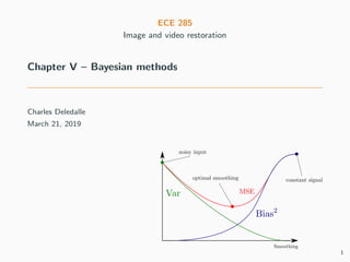
  • 24. Mean square error – Bias and Variance MSE(x, ˆx) = ||x − E[ˆx]||2 Bias2 + tr Var[ˆx] Variance In general, the minimum MSE estimator has non-zero bias and non-zero variance Figure 1 – Smoothing more ⇒ increasing bias while reducing variance 21
  • 25. Mean square error – Optimal estimation Optimize for a class of estimators • Choose the optimal estimator as the one minimizing the expected loss ˆx = argmin ˆx∈C {R(x, ˆx) = E[ (x, ˆx)]} for C a class of estimators. • Without this restriction, solutions can be unrealizable, ex: trivial solution ˆx(y1 , . . . , ym ) = x i.e., the solution would depend on the unknown. 22
  • 26. Mean square error – Optimal estimation Example (Amplified sample mean (1/3)) • Assume yk iid with E[yk ] = x and Var[yk ] = σ2 Idn. • Consider the optimal estimator with respect to the MSE ˆx = argmin ˆx∈C MSE(x, ˆx) = E||x − ˆx||2 2 • And the class of functions that amplify the sample mean C =    ˆx : Rn × . . . × Rn m times → Rn ; ∃α ∈ R, ˆx(y1 , . . . , ym ) = α m m k=1 yk    • Finding ˆx leads to find α that minimizes the MSE. 23
  • 27. Mean square error – Optimal estimation ˆx(y1 , . . . , ym ) = α m m k=1 yk Example (Amplified sample mean (2/3)) • Study the first order derivative ∂MSE(x, ˆx) ∂α = ∂||x − E[ˆx(y)]||2 2 ∂α + ∂ tr Var [ˆx(y)] ∂α = ∂||x − αx||2 2 ∂α + ∂α2 tr Var [y] /m ∂α = ||x||2 ∂(1 − α)2 ∂α + nσ2 m ∂α2 ∂α = −2||x||2 (1 − α) + 2n m σ2 α • Moreover, the second order derivative is constant and positive ∂2 MSE ∂α2 = 2||x||2 + 2n m σ2 24
  • 28. Mean square error – Optimal estimation Example (Amplified sample mean (3/3)) • Then the MSE is a quadratic function and its minimum is given for ∂MSE ∂α = 0 ⇔ −2||x||2 (1 − α) + 2n m σ2 α = 0 ⇔ α = ||x||2 ||x||2 + nσ2 m Define: SNR2 = ||x||2 2 nσ2 α = SNR2 SNR2+1/m : • large SNR, yk has good quality, average: ˆx = ¯y, • low SNR, x drawn in the noise: ˆx = 0 is safer. This is not realizable since it depends on the unknown x. We need an alternative to direct MSE minimization. 25
  • 30. Unbiased estimators – Minimum Variance Unbiased Estimator • In the previous example ∂MSE(x, ˆx) ∂α = ∂Bias2 ∂α + ∂Variance ∂α where ∂Bias2 ∂α = −2||x||2 (1 − α) and ∂Variance ∂α = 2n m σ2 α • The dependency on ||x||2 arises from the bias term, • This occurs in many situations. Constrain the estimator to be unbiased. Find the estimator that produces the minimum variance. This will provides the minimum MSE among all unbiased estimators. 26
  • 31. Unbiased estimators – Minimum Variance Unbiased Estimator Minimum Variance Unbiased Estimator (MVUE) An estimator ˆx ∈ C is the MVUE for the class of estimators C if (∀x, Eˆx = x) unbiasedness and ∀˜x ∈ C, (∀x, E˜x = x) ⇒ (∀x, tr Var[ˆx ] tr Var[˜x]) minimum variance Example (Back to the amplified sample mean) • An unbiased estimator that amplifies the sample mean should satisfy Bias2 = ||x − E α m m k=1 yk ||2 = (1 − α)2 ||x||2 = 0 ⇒ α = 1 • Then the sample mean is the only unbiased estimator of this class. • It is the MVUE of this class. 27
  • 32. Unbiased estimators – Minimum Variance Unbiased Estimator Variance of 3 unbiased estimators E[ˆx1 ]=E[ˆx2 ]=E[ˆx3 ]=x as a function of x. Quiz: which one is the MVUE on the left? on the right? The MVUE does not always exist. If it does exist, how to find it? 28
  • 33. Unbiased estimators – Cram´er-Rao bound Cram´er-Rao lower bound (≈ 1945) • Provided the bound exists, any realizable unbiased estimator satisfies Var[ˆx] I−1 where Ii,j = E ∂2 − log p(y1 , . . . , ym ; x) ∂xi∂xj x • Var[ˆx] I−1 means Var[ˆx] − I−1 is symmetric positive definite, • y1 , . . . , ym → p(y1 , . . . , ym ; x) is the law of the observations, • x → p(y1 , . . . , ym ; x) is the likelihood of the unknown, • I the Fisher information matrix: expected Hessian of the log-likelihood, • I measures the organization/entropy/simplicity of the problem, • Ex: small noise → likelihood peaky → large Hessian → small bound. 29
  • 34. Unbiased estimators – Cram´er-Rao bound Consequence: Var[ˆx] = I−1 ⇒ ˆx is the MVUE If you find an unbiased estimator that reaches the Cram´er-Rao bound, then it is the MVUE. The MVUE may not reach the Cram´er-Rao bound, in this case, no estimator reaches the bound. 30
  • 35. Unbiased estimators – Efficiency Efficiency • The ratio 0 tr I−1 tr Var[ˆx] 1 is called efficiency of the estimator, • Measures by how much the estimator is close to the Cram´er-Rao bound, • An unbiased estimator with efficiency 100% is said to be efficient, • If an efficient estimator exists, it is the MVUE, • The MVUE is not necessarily efficient. If we cannot build an efficient estimator, we may build one whose efficiency converges to 100% with the number of observations m. 31
  • 36. Unbiased estimators – Maximum Likelihood Estimator Maximum likelihood estimators (MLE) [Fisher, 1913 and others] • Define the MLE, for yk iid, as one of the global minima of the likelihood ˆx ∈ argmax x p(y1 , . . . , ym ; x) = argmax x m k=1 p(yk ; x) • Then ˆx is asymptotically unbiased, asymptotically efficient and consistent lim m→∞ E[ˆx] = x, lim m→∞ Var[ˆx] = 0, plim m→∞ ˆx = x and lim m→∞ tr I−1 tr Var[ˆx] = 1 • If an efficient estimator exists, it is the MLE and, then, the MVUE. • Otherwise, the MVUE might be more efficient than the MLE. MLE: look for the image that best explains the observations. 32
  • 37. Unbiased estimators – Maximum Likelihood Estimator 0 2 4 6 8 10 0 0.05 0.1 0.15 0.2 0.25 (a) Gaussian likelihood 0 2 4 6 8 10 0 0.05 0.1 0.15 0.2 0.25 0.3 0.35 0.4 (b) Laplace likelihood 0 2 4 6 8 10 0 0.1 0.2 0.3 0.4 0.5 (c) Cauchy likelihood 0 2 4 6 8 10 0 0.1 0.2 0.3 0.4 0.5 (d) Poisson likelihood 0 2 4 6 8 10 0 0.1 0.2 0.3 0.4 0.5 0.6 (e) Gamma likelihood 0 2 4 6 8 10 0 0.1 0.2 0.3 0.4 0.5 0.6 (f) Impulse likelihood • These curves are not laws but likelihoods: x → p(y1 , . . . , ym ; x). • The considered samples are yk = 4, 10, 3, 6, 2, 3, 2, 2, 4. • MLE can be the sample mean, median, mode, or something else. 33
  • 38. Unbiased estimators – Maximum Likelihood Estimator How to find the MLE for yk iid? • Rewrite the MLE as a minimization problem ˆx ∈ argmax x m k=1 p(yk ; x) = argmin x m k=1 − log p(yk ; x) ˆ(x) • Why − log? • Strictly decreasing function: same locations for the optima, • Sums are easier to manipulate than products, • p(yk ; x) very small: safer to manipulate −16 than 10−16 . 34
  • 39. Unbiased estimators – Maximum Likelihood Estimator How to find the MLE for yk iid? • If ˆ differentiable: find ˆx that cancels the gradient • Twice diff. at ˆx and ˆ (ˆx ) > 0: a local minimum • ˆ convex: a global minimum ˆ(αx + βy) αˆ(x) + βˆ(y) • Twice diff. everywhere and ˆ (x) 0: ˆ convex ⇒ a global minimum • Often analytical solutions, otherwise use numerical solvers (ex: Gradient descent, Newton-Raphson, Expectation-Maximization) In multivariate setting, ˆ (x) > 0 means the Hessian is symmetric positive definite at x. 35
  • 40. Unbiased estimators – Maximum Likelihood Estimator Example (Poisson noise (1/3)) • Consider samples y1 , . . . , ym ∈ N iid versions of x 0 such that p(y; x) = xy e−x y! • We have ˆ(x) = m k=1 − log p(yk ; x) = m k=1 −yk log x + x − log yk ! 36
  • 41. Unbiased estimators – Maximum Likelihood Estimator Example (Poisson noise (1/3)) • Consider samples y1 , . . . , ym ∈ N iid versions of x 0 such that p(y; x) = xy e−x y! • We have ˆ(x) = m k=1 − log p(yk ; x) = m k=1 −yk log x + x − log yk ! • It follows that ˆ is twice differentiable and ˆ(x) = m k=1 − yk x + 1 = m − 1 x m k=1 yk and ˆ (x) = 1 x2 m k=1 yk 36
  • 42. Unbiased estimators – Maximum Likelihood Estimator Example (Poisson noise (1/3)) • Consider samples y1 , . . . , ym ∈ N iid versions of x 0 such that p(y; x) = xy e−x y! • We have ˆ(x) = m k=1 − log p(yk ; x) = m k=1 −yk log x + x − log yk ! • It follows that ˆ is twice differentiable and ˆ(x) = m k=1 − yk x + 1 = m − 1 x m k=1 yk and ˆ (x) = 1 x2 m k=1 yk • For all x, ˆ (x) > 0, then ˆ is convex and thus ˆx satisfies m − 1 ˆx m k=1 yk = 0 ⇔ ˆx = 1 m m k=1 yk 36
  • 43. Unbiased estimators – Maximum Likelihood Estimator Example (Poisson noise (2/3)) • The MLE for Poisson noise is unique and is the sample mean, • Recall that for Poisson noise E[yk ] = x and Var[yk ] = x, • It follows that the variance of the MLE is Var[ˆx ] = 1 m2 m k=1 Var[yk ] = 1 m2 m k=1 x = x m 37
  • 44. Unbiased estimators – Maximum Likelihood Estimator Example (Poisson noise (2/3)) • The MLE for Poisson noise is unique and is the sample mean, • Recall that for Poisson noise E[yk ] = x and Var[yk ] = x, • It follows that the variance of the MLE is Var[ˆx ] = 1 m2 m k=1 Var[yk ] = 1 m2 m k=1 x = x m • Besides, the Fisher information is I = E[ˆ (x)] = E 1 x2 m k=1 yk = 1 x2 m k=1 E[yk ] = 1 x2 m k=1 x = m x 37
  • 45. Unbiased estimators – Maximum Likelihood Estimator Example (Poisson noise (2/3)) • The MLE for Poisson noise is unique and is the sample mean, • Recall that for Poisson noise E[yk ] = x and Var[yk ] = x, • It follows that the variance of the MLE is Var[ˆx ] = 1 m2 m k=1 Var[yk ] = 1 m2 m k=1 x = x m • Besides, the Fisher information is I = E[ˆ (x)] = E 1 x2 m k=1 yk = 1 x2 m k=1 E[yk ] = 1 x2 m k=1 x = m x • Hence Var[ˆx ] = I−1 • The MLE reaches the Cram´er-Rao, even non-asymptotically. • It is 100% efficient for all m, it’s the MVUE. 37
  • 46. Unbiased estimators – Maximum Likelihood Estimator Law MLE Comments MVUE Gaussian Sample mean 100% efficient for all m √ (sample median ≈ 64%) Poisson Sample mean 100% efficient for all m √ Gamma Sample mean 100% efficient for all m √ Cauchy No closed form (sample median ≈ 81%) (24%-trimmed mean ≈ 88%) Laplacian Sample median asymptotically efficient with m Impulse Sample mode no CR bound Remarks: robust estimators • Even though the sample mean is often the MLE, the sample median (which always converges) or the trimmed mean are often preferred when the noise distribution is unknown or known approximately. (their efficiency often drops slower under mis-specified noise models) • More robust to outliers, when some samples are not iid. 38
  • 48. Least square – Best Linear Unbiased Estimator Motivation: • The MVUE not always exist, • Can be difficult to find. Idea:    • Restrict the estimator to be linear with respect to y, • Restrict the estimator to be unbiased, • Find the best one (i.e., with minimum variance) Definition (BLUE: Best linear unbiased estimator) • Consider yk ∈ Rn and x ∈ Rp , • BLUE is the MVUE for the class of linear estimators C = ˆx ; ∃A1, . . . , Am ∈ Rp×n , ˆx(y1 , . . . , ym ) = m k=1 Akyk 39
  • 49. Least square – Best Linear Unbiased Estimator Theorem (Gauss-Markov theorem) • Assume • H ∈ Rn×p with rank p n (i.e., over-determined) • E[yk ] = Hx • Var[yk ] = Σ • Then, the BLUE is ˆx = (H∗ Σ−1 H)−1 H∗ Σ−1 ¯y where ¯y = 1 m m k=1 yk . • BLUE always exists for over-determined linear regression problems, • Can be used even though we do not know precisely p(y1 , . . . , ym ; x) as: It only requires the noise to be zero-mean, and knowing its covariance matrix. • H∗ Σ−1 H is always sdp ⇒ can be inverted by conjugate gradient. 40
  • 50. Least square – Best Linear Unbiased Estimator MLE with Gaussian noise = BLUE = LSE • Assume • H ∈ Rn×p with rank p n (i.e., over-determined), • yk ∼ N(Hx, Σ) and independent. • Then, the MLE is unique and is the least square estimator (LSE) x = argmin x m k=1 ||Σ−1/2 (Hx − yk )||2 2 = (H∗ Σ−1 H)−1 H∗ Σ−1 ¯y • It is also the BLUE and the MVUE. Imposing linearity and unbiasedness (sub-optimal in general) ≡ Imposing unbiasedness and assuming Gaussianity. (optimal under this assumption) 41
  • 51. Least square – Least square for super-resolution Σ = σ2 Id ˆx = (H∗ H)−1 H∗ ¯y p1, p2 = x.shape[:2] sigma = 60/255 m = 20 # Subsampling: each line is the average of two consecutive ones H = lambda x: (x[0::2, :] + x[1::2, :]) / 2 y = [ H(x) + sigma * np.random.randn(int(p1 / 2), p2, 3) for k in range(m) ] # Adjoint of H: each line is duplicated and divided by two Ha = lambda x: x[[int(i/2) for i in range(p1)], :] / 2 # Least square solution with cgs (Note: non optimal) ybar = np.mean(y, axis=0) xblue = im.cg(lambda x: Ha(H(x)), Ha(ybar)) (a) yk = Hx + wk (b) ˆx , m = 1 (c) ˆx , m = 4 (d) ˆx , m = 20 42
  • 52. Least square – Under-determined least square Oops, we have not check that H∗ H was invertible. In image processing tasks • H is almost always under-determined ⇒ H∗ H is non-invertible. Examples • Low-pass: sets high frequencies to zero, thus non-invertible, • Radon transform: sets some frequencies to zero, thus non-invertible, • Inpainting: sets some pixels to zero, thus non-invertible, • Super-resolution: p > n the problem is under-determined. If H is non-invertible, BLUE does not exist. Realizable estimators cannot be unbiased. They cannot guess, not even in average, what was lost. 43
  • 53. Least square – Least square and normal equation So, what was cgs computing in the previous example? Least-square estimator and normal equation • cgs finds one of the infinite solutions of the least square problem x ∈ argmin x ||Hx − ¯y||2 2 • They are characterized by the normal equation H∗ Hx = H∗ ¯y • If initialized to zero, cgs finds the one with minimum norm ||ˆx ||2. • This solution reads as ˆx = H+ ¯y where H+ ∈ Rp×n is the Moore-Penrose pseudo-inverse of H. 44
  • 54. Least square – Least square and normal equation Moore-Penrose pseudo-inverse • The Moore-Penrose pseudo-inverse is the unique matrix satisfying 1 HH+ H = H 2 H+ HH+ = H+ 3 (HH+ )∗ = HH+ 4 (H+ H)∗ = H+ H • The Moore-Penrose pseudo-inverse always exists. • If H is square and invertible: H+ = H−1 • H+ also satisfy: H+ = (H∗ H)+ H∗ = H∗ (HH∗ )+ • If H has full rank: H+ =(H∗ H)−1 H∗ , we recover Gauss-Markov thm. 45
  • 55. Least square – Moore-Penrose pseudo-inverse Small detour to Singular Value Decompositions (SVD) • Any matrix H ∈ Rn×m admits a Singular Value Decomposition (SVD) as H = UΣV ∗ with    • U ∈ Cn×n , U∗ U = U∗ U = Idn • V ∈ Cm×m , V ∗ V = V V ∗ = Idm • Σ ∈ Rn×m a diagonal matrix. • σi = Σii > 0: called singular values (often sorted in decreasing order), • Rank r min(n, m): number of non-zero singular values. 46
  • 56. Least square – Moore-Penrose pseudo-inverse SVD, image and null space • If the singular values are sorted in decreasing order Im[H] = {y ∈ Rn ; ∃x ∈ Rm , y = Hx} = Span({ui ∈ Rn ; i ∈ [1 . . . r]}) (what can be observed) Ker[H] = {x ∈ Rm ; Hx = 0} = Span({vi ∈ Rm ; i ∈ [r + 1 . . . m]}) (what is lost) where ui are the columns of U and vi are the columns of V Null-space: set of zero-frequencies, set of missing pixels, ... 47
  • 57. Least square – Moore-Penrose pseudo-inverse SVD and Moore-Penrose pseudo-inverse • Let H = UΣV ∗ be its SVD, the Moore-Penrose pseudo inverse is H+ = V Σ+ U∗ where σ+ i = 1 σi if σi > 0 0 otherwise • For deconvolution: SVD ∼= eigendecomposition ∼= Fourier decomposition ⇒ inversion of the non-zero frequencies. • Difficulty: 1 σi can be very large (ill-conditioned matrix) ⇒ numerical issues (refer to assignment 7). Compared to other least square solutions, the Moore-Penrose pseudo-inverse does not create new content in Ker[H], i.e., where the information was lost. It is unbiased only on Ker[H]⊥ . 48
  • 58. Least square – Pseudo inverse for deconvolution In practice, the threshold 1e-2 is difficult to choose n1, n2 = x.shape[:2] sigma = 2/255 m = 20 # Deconvolution problem setting nu = im.kernel('gaussian', tau=2, s1=20, s2=20) lbd = im.kernel2fft(nu, n1, n2) H = lambda x: im.convolvefft(x, lbd) y = [ H(x) + sigma * np.random.randn(n1, n2, 3) for i in range(m) ] # Numerical Fourier approximation of the pseudo inverse lbd_pinv = 1 / lbd lbd_pinv[np.abs(lbd) < 1e-2] = 0 ybar = np.mean(y, axis=0) x_pinv = im.convolvefft(ybar, lbd_pinv) (a) yk (b) m = 1 (c) m = 10 (d) m = 20 49
  • 59. Least square and unbiased estimator issues The M.-P. pseudo-inverse does not create new content on Ker[H], it cannot recover missing information Moreover, unbiased estimators amplify and colorize noise. −−−−−−−−−→ PINV/LSE/MLE/MVUE • In practice, the number m of samples/frames/views is small, • The asymptotic behavior when m → ∞ is far from being reached, • In fact, in our contexts of interest, we often have m = 1. 50
  • 61. Bayesian approach – Motivations Why unbiased estimators are not working in our context? Because they attempt to be optimal whatever the underlying image x. Bayesian answer: Forget about unbiasedness and be optimal only for the class of images x that looks like clean images. Expected behavior: If x looks like a clean image: small bias, small variance. If x does not look like a clean image: large bias and/or large variance. 51
  • 62. Bayesian approach – Random vector models Observed image y ∈ Rn (n pixels): random vector with density p(y) = p(y, x) dx = p(y|x)p(x) dx (Marginalization) where x ∈ Rn is also a random vector modeling clean images. • p(y|x) degradation model – law of y|x – likelihood of x|y • p(x) prior distribution of x • p(y) marginal distribution of y 52
  • 63. Bayesian approach – How to choose the likelihood? Modeling the likelihood p(y|x) (relatively easy) • Based on the knowledge of the acquisition process • Linear additive model: y = Hx + w • Multiplicative noise: y = x × w • Poisson noise: p(y|x) = xy e−x y! • White noise: E[w] = 0 and Var[w] diagonal 53
  • 64. Bayesian approach – How to choose the prior? Modeling the prior p(x) (hard) • Based on your prior knowledge of the underlying signal • Are clean images piece-wise smooth? simple? observable on the web? . . . x = ? Try to cover as many cases as possible without covering bad images. The prior should help at separating signal and noise. 54
  • 65. Bayesian approach – Framework Bayesian approach • Model the likelihood: p(y | x), • Choose a prior: p(x), • Estimate the posterior distribution based on Bayes rule: p(x | y) = p(y | x)p(x) p(y) i.e, Posterior = Likelihood × Prior Marginal 55
  • 66. Bayesian approach – Posterior mean Posterior mean • Compute the mean of the posterior, or posterior mean x = E[x|y] = xp(x | y) dx • Potentially, compute the posterior variance Var[x|y] = (x − E[x|y])(x − E[x|y])∗ p(x | y) dx to build regions of confidence, and account for uncertainty. 56
  • 67. Bayesian approach – MAP or Maximum a Posteriori (MAP) • Take a mode of the posterior, or Maximum a Posteriori x ∈ argmax x p(x | y) 57
  • 69. Posterior mean Posterior mean depends only on the likelihood and the prior ˆx(y) = E[x | y] = xp(x|y) dx = xp(y|x)p(x) dx p(y) = xp(y|x)p(x) dx p(y, x) dx = xp(y|x)p(x) dx p(y|x)p(x) dx Posterior mean is always realizable. 58
  • 70. Posterior mean Bayesian MSE As x is random, the mean square error (MSE) is defined as a double integral MSE(ˆx) = E[||x − ˆx||2 2] = ||x − ˆx(y)||2 2 p(y, x) dy dx Theorem (Optimality of the posterior mean) The Minimum (Bayesian) MSE estimator (MMSE) is unique and given by the posterior mean ˆx = argmin ˆx MSE(ˆx) = E[x | y] = xp(x | y) dx The posterior mean ˆx is the estimator that is as close as possible to x, on average for likely clean images x and their corrupted versions y. 59
  • 71. Posterior mean – Proof Lemma – Conditional expectation. E[f(x)] = f(x)p(x) dx = f(x)p(x, y) dx dy = f(x)p(x|y)p(y) dx dy = f(x)p(x|y) dx p(y) dy = E[f(x) | y] p(y) dy = E {E[f(x)|y]} 60
  • 72. Posterior mean – Proof Proof. The previous Lemma leads to E[||x − ˆx(y)||2 2] = E E[||x − ˆx(y)||2 2 | y] = E[||x − ˆx(y)||2 2 | y] p(y) dy This quantity is minimal if, for all y, we have ˆx(y) ∈ argmin z E[||x − z||2 2 | y] Given y, we have to minimize with respect to z the quantity E[||x − z||2 2 | y] = E[||x||2 | y] + ||z||2 − 2 z, E[x | y] By linearity, the first order optimality condition gives 2E[x | y] − 2z = 0 ⇔ z = E[x | y] 61
  • 73. Posterior mean • Optimal in the MMSE sense • In general, difficult integration problem • Explicit solutions in few cases (see, conjugate priors) E[x | y] = xp(y|x)p(x) dx p(y|x)p(x) dx If no explicit solutions, several workarounds: 1 LMMSE estimator: Restrict to linear estimators. 2 Wiener estimator: Restrict to LTI estimators. 3 Monte-Carlo estimator: Estimate E[x | y] from a data-set. 4 MCMC/Metropolis Hastings: Otherwise. 62
  • 75. Maximum A Posteriori (MAP) estimator Forget about the optimality of the MMSE, and instead of taking the posterior mean, take the posterior mode. Maximum A Posteriori (MAP) estimator ˆx(y) ∈ argmax x p(x | y) = argmax x p(y|x)p(x) p(y) = argmax x p(y|x)p(x) As for the posterior mean, the MAP depends only on the likelihood and the prior. 63
  • 76. Maximum A Posteriori (MAP) estimator Maximum A Posteriori (MAP) estimator • The MAP is connected with variational methods: ˆx(y) ∈ argmax x p(y|x) Likelihood p(x) prior = argmin x − log p(y|x) Data fit − log p(x) Regularisation 64
  • 77. Maximum A Posteriori (MAP) estimator MMSE xp(y|x)p(x) dx p(y|x)p(x) dx Integration problem vs MAP argmax x p(y|x)p(x) Optimization problem • Integration can be intractable and/or leads to long computation time. • Optimization is often simpler and faster (does not mean straightforward). • We will see several examples later. But first, when do both estimators coincide? 65
  • 78. Linear Minimum Mean Square Error
  • 79. LMMSE estimator – Optimal linear filtering Linear Minimum Mean Square Error (LMMSE) • Let y ∈ Rn and x ∈ Rp be two random vectors such that E[y | x] = Hx and Var[y | x] = Σ E[x] = µ and Var[x] = L • Consider the class of affine estimators C = ˆx ; ∃A ∈ Rp×n , b ∈ Rp , ˆx(y) = Ay + b • The LMMSE estimator is ˆx = argmin ˆx∈C E[||x − ˆx||2 2] = µ + LH∗ (HLH∗ + Σ)−1 (y − Hµ) • Unlike BLUE, H can be under-determined here because L and Σ are always sdp, hence invertible. 66
  • 80. LMMSE estimator – Optimal linear filtering As for the BLUE, the LMMSE depends only on the means and variances 67
  • 81. LMMSE estimator – Optimal linear filtering MAP with Gaussian models = LMMSE = Penalized Least Square • Let y ∈ Rn and x ∈ Rp be independent and such that y|x ∼ N(Hx, Σ) x ∼ N(µ, L) • Then, the MAP is a penalized least square estimator (PLSE) ˆx = argmin ˆx − log p(y|ˆx) − log p(ˆx) = argmin ˆx ||Σ−1/2 (y − Hˆx)||2 2 Data fit + ||L−1/2 (ˆx − µ)||2 2 Penalization = µ + (H∗ Σ−1 H + L−1 )−1 H∗ Σ−1 (y − Hµ) (Null gradient) = µ + LH∗ (HLH∗ + Σ)−1 (y − Hµ) (Woodbury) • It is also the MMSE and the LMMSE. 68
  • 82. LMMSE estimator – Optimal linear filtering LMMSE under white noise • For simplicity add the restriction that the noise is white Var[y | x] = Σ = σ2 Id • In this case the LMMSE has a simplified expression ˆx = argmin ˆx 1 σ2 ||y − Hˆx||2 2 + ||L−1/2 (ˆx − µ)||2 2 = µ + (H∗ H + σ2 L)−1 H∗ (y − Hµ) • H∗ H + σ2 L−1 always invertible and symmetric positive definite (you can always use conjugate gradient ) 69
  • 83. LMMSE estimator – Optimal linear filtering ˆx = µ + (H∗ H + σ2 L−1 )−1 H∗ (y − Hµ) LMMSE vs BLUE • Define SNR2 = tr L nσ2 = Uncertainty on the signal Variation of the noise • If H over-determined, the LMMSE tends to the BLUE (least square) lim SNR→∞ ˆx = µ + (H∗ H)−1 H∗ (y − Hµ) = µ + (H∗ H)−1 H∗ y − (H∗ H)−1 H∗ Hµ µ = (H∗ H)−1 H∗ y = H+ y As you try to be uniformly optimal for all x (maximal uncertainty) you will fail at restoring y, all the more as you have noise. 70
  • 84. LMMSE estimator – Optimal linear filtering LMMSE for denoising • If moreover H = Id (denoising problem), this simplifies as ˆx = argmin ˆx 1 σ2 ||y − ˆx||2 2 + ||L−1/2 (ˆx − µ)||2 2 = µ + L(L + σ2 Id)−1 (y − µ) Let us pick some µ and L and try this formula for denoising. 71
  • 85. LMMSE estimator – Optimal linear filtering Example (Lets pick a naive model) • Consider y = x + w ∈ Rn with x and w independent such that E[y | x] = x and Var[y | x] = σ2 Idn, E[x] = 0 and Var[x] = L = λ2 Idn. • Then the LMMSE filter reads as ˆx = µ + L(L + σ2 Id)−1 (y − µ) = 0 + λ2 (λ2 Id + σ2 Id)−1 (y − 0) = λ2 λ2 + σ2 y = SNR2 SNR2 + 1 y with SNR2 = λ2 σ2 • It’s similar to the optimal amplified estimator except this one is realizable. 72
  • 86. LMMSE estimator – Naive model – Limitations (a) x (unknown) (b) y (observation) (c) ˆx (estimate) Limitations of this naive model • Amplifying the noisy input will never allow us removing noise, • Would work only if all clean images were like pure white noise. 73
  • 87. LMMSE estimator – Naive model – Limitations (a) We assumed x to be likely somewhere here. (b) but it was somewhere there. Limitations of this naive model • Images contain structures that must be captured by µ and L, • Goal: define/find the ellipsoid localizing x with high probability, • How: make use of the eigendecomposition: L = EΛE∗ . 74
  • 88. LMMSE estimator – Filtering in the eigenspace ˆx = µ + L(L + σ2 Id)−1 (y − µ) • Consider the eigendecomposition: L = EΛE∗ , then L(L + σ2 Idn)−1 = E          λ2 1 λ2 1+σ2 0 λ2 2 λ2 2+σ2 ... 0 λ2 n λ2 n+σ2          E∗ ⇒ The LMMSE filter can be re-written as ˆx = µ + Eˆz Come back where ˆzi = λ2 i λ2 i + σ2 zi shrinkage and z = E∗ (y − µ) Change of origin and basis • Shrinkage adapts to the SNR in each eigendirection: SNR2 i = λ2 i /σ2 . What representation (µ and E)? What shrinkage (Λ)? 75
  • 90. Wiener filtering – Whitening via the Fourier transform Whitening Let L−1/2 = Λ−1/2 E∗ . Let x be a random variable. Then E[x] = µ and Var[x] = L if and only if η = L−1/2 (x − µ) with E[η] = 0 and Var[η] = Idn 76
  • 91. Wiener filtering – Whitening via the Fourier transform L−1/2 (x−µ) −−−−→ Modeling the two first moments of x ≡ Find the affine transform that makes it look like white noise What kind of transform can make typical images white? 77
  • 92. Wiener filtering – Whitening via the Fourier transform Whitening using DFT • Assume Fourier coefficients to be decorrelated, • Choose µ = 0 and L = EΛE−1 with E = 1 √ n         ×n         DFT: F ←−−−− Columns form the Fourier basis E−1 = √ nF −1 Λ = diagonal, real and positive (L is sdp) 78
  • 93. Wiener filtering – Whitening via the Fourier transform Whitening using DFT • E and µ fixed: L = Cov[x] ⇔ Λ = Var[E∗ (x − µ)] • In our case: λ2 i = n−1 × E[|(F x)i|2 ] = mean power spectral density = variance for each frequency 79
  • 94. Wiener filtering – Whitening via the Fourier transform Mean power spectral density Si = E[|(F x)i|2 ] • Estimate it from a collection of clean images x1, x2, . . . • Use a model to reduce its degree of freedom [Van der Schaafa et al., 1996] Si = neβ ui n1 2 + vi n2 2 α . • Estimate α and β by least square in log-log (see assignment). • Arbitrary zero frequency (DC component): its variance goes to infinity. 80
  • 95. Wiener filtering – Whitening via the Fourier transform Prior localization for clean images 81
  • 96. Wiener filtering – Denoising Wiener filter for denoising • In denoising, this LMMSE is called Wiener filter and reads ˆx = F −1 ˆz iDFT where ˆzi = λ2 i λ2 i + σ2 zi shrink each frequency and z = F y DFT • Using λ0 → ∞: DC is unchanged. (a) y = x + w (b) z (c) λ2 i λ2 i +σ2 (d) ˆz (e) ˆx 82
  • 97. Wiener filtering – Denoising Results of Wiener filtering in denoising (a) y (b) z (c) λ2 i λ2 i +σ2 (d) ˆz (e) ˆx y = x + sigma * np.random.randn(x.shape) z = nf.fft2(y, axes=(0, 1)) zhat = lbd**2 / (lbd**2+ sigma**2) * z xhat = np.real(nf.ifft2(zhat, axes=(0, 1))) z = √ n −1 Fy ˆzi = λ2 i λ2 i + σ2 zi ˆx = √ nF−1 ˆz The technique auto-adapts to the noise level Results are blurry, too smooth 83
  • 98. Wiener filtering – Denoising Results of Wiener filtering in denoising (a) y (b) z (c) λ2 i λ2 i +σ2 (d) ˆz (e) ˆx y = x + sigma * np.random.randn(x.shape) z = nf.fft2(y, axes=(0, 1)) zhat = lbd**2 / (lbd**2+ sigma**2) * z xhat = np.real(nf.ifft2(zhat, axes=(0, 1))) z = √ n −1 Fy ˆzi = λ2 i λ2 i + σ2 zi ˆx = √ nF−1 ˆz The technique auto-adapts to the noise level Results are blurry, too smooth 83
  • 99. Wiener filtering – Denoising Results of Wiener filtering in denoising (a) y (b) z (c) λ2 i λ2 i +σ2 (d) ˆz (e) ˆx y = x + sigma * np.random.randn(x.shape) z = nf.fft2(y, axes=(0, 1)) zhat = lbd**2 / (lbd**2+ sigma**2) * z xhat = np.real(nf.ifft2(zhat, axes=(0, 1))) z = √ n −1 Fy ˆzi = λ2 i λ2 i + σ2 zi ˆx = √ nF−1 ˆz The technique auto-adapts to the noise level Results are blurry, too smooth 83
  • 100. Wiener filtering – Limits and connections to LTI filters Wiener filtering for denoising ˆzi = λ2 i λ2 i + σ2 zi elementwise product ⇔ ˆx = ν ∗ y convolution ≡ moving average • Wiener filter: optimal LTI filter in the Bayesian MMSE sense, ⇒ It is a low-pass filter, i.e., a weighted average. -30 -20 -10 0 10 20 30 0 0.005 0.01 0.015 0.02 0.025 Heat/Gauss kernel Wiener kernel 84
  • 101. Wiener filtering – Application to deconvolution Wiener deconvolution • For deconvolution, the LMMSE filter reads as ˆx = µ + (H∗ H + σ2 L−1 )−1 H∗ (y − µ) with H a circulant matrix: H = F −1 ΩF with Ω = diag(ω1, . . . , ωn). • We get that ˆx = (F −1 Ω∗ F F −1 ΩF + σ2 F −1 Λ−1 F )−1 F −1 Ω∗ F y = F −1 (Ω∗ Ω + σ2 Λ−1 )−1 Ω∗ F y • Or equivalently ˆx = F −1 ˆz where ˆzi = ω∗ i |ωi|2 + σ2/λ2 i zi and z = F y • Filter adapts to the SNR for each frequency. 85
  • 102. Wiener filtering – Application to deconvolution (a) y (b) z (c) ω∗ i |ωi|2+σ2/λ2 i (d) ˆz (e) ˆx Wiener deconvolution: optimal spectral sharpening. 86
  • 103. Wiener filtering – Application to deconvolution Wiener versus pseudo inverse (a) Observation y (b) PINV H+ y (c) Wiener ˆx Invert attenuated frequencies while preventing from amplifying the noise. 87
  • 104. Wiener filtering – Application to deconvolution Wiener versus pseudo inverse (a) Observation y (b) PINV H+ y (c) Wiener ˆx Invert attenuated frequencies while preventing from amplifying the noise. 87
  • 105. Learning the LMMSE filter with PCA
  • 106. LMMSE + Learning with PCA Can we instead learn the ellipsoid (µ and L)? Use an external data-set • Let x1, . . . , xk be a collection of images. • Estimate µ = E[xk] and L = Var[xk] from the samples µ = 1 K K k=1 xk and L = 1 K − 1 K k=1 (xk − µ)(xk − µ)∗ • Problem: computing L requires to store n2 values, • For an image of size n = 256 × 256 n2 = 4, 294, 967, 296 (16Gb in single precision) 88
  • 107. LMMSE + Learning with PCA Use SVD • Let ˜xk = xk − µ and ˜X = 1√ K−1 ˜x1 . . . ˜xK , we have L = 1 K − 1 K k=1 (xk − µ)(xk − µ)∗ = ˜X ˜X∗ • The SVD of ˜X reads ˜X = EΛ1/2 V ∗ for some V ∗ =V −1 . Proof: L = ˜X ˜X∗ = EΛ1/2 V ∗ V Λ1/2 E∗ = EΛE∗ • The SVD decomposition of ˜X gives E and Λ. • No need to build ˜X ˜X∗ , but still E is a n × n matrix (16 Gb) 89
  • 108. LMMSE + Learning with PCA Low rank property • ˜X is a n × K matrix (K < n), whose columns are zero on average: 1 K K k=1 ˜xk = 1 K K k=1 (xk − µ) = 1 K K k=1 xk − µ = 0 • One of the columns is a linear combination of the others K k=1 ˜xk = 0 ⇔ ˜x1 = − K k=2 ˜xk • The family {˜xk } has K − 1 independent vectors. • The rank of ˜X is r = K − 1. How does that help? 90
  • 109. LMMSE + Learning with PCA Reduced SVD • ˜X has only r non-zero singular values ˜X = EΛ1/2 V ∗ = E1 E0 Λ 1/2 1 0 0 0 V ∗ 1 V ∗ 0 = E1Λ 1/2 1 V ∗ 1 • L has only r non-zero eigenvalues and depends only on E1 and Λ1 L = EΛE∗ = E1 E0 Λ1 0 0 0 E∗ 1 E∗ 0 = E1Λ1E∗ 1 Require to store only n × r + r values (r vectors ei ∈ Rn + r values λi ∈ R+ ) 91
  • 110. LMMSE + Learning with PCA Principle component analysis (PCA) • Assume the rank r being K − 1 or even lower L = EΛE∗ = E1Λ1E∗ 1 = r i=1 λ2 i eie∗ i ⇒ Clean images are a linear combination of a few r images x = µ + L1/2 η = µ + r i=1 ηiλiei with controlled weights E[ηi] = 0 and Var[ηi] = 1. • The r directions ei are called principle direction. • Best way to capture most of variability with r dimensions only, i.e., to cover most of the clean images with limited memory. 92
  • 111. LMMSE + Learning with PCA Example (Face dataset with additive white Gaussian noise) • AT&T Database of Faces http://www.cl.cam.ac.uk/research/dtg/attarchive/facedatabase.html • 40 subjects, 10 images per subject (400 images in total) • Gray-scale images of size 92 × 112 = 10304 pixels • 39 subjects for the xk and 1 subject for y = x + w X = (x1, . . . , xK ) =    , , , , , ×390 , . . .    y = = + , w ∼ N(0, σ2 Idn) 93
  • 112. LMMSE + Learning with PCA – Example X =   , , , , , ×390 , . . .   import numpy.linalg as nl # Learning step (K = 390 files) fs = [ 'filetrain1.png', ... ] X = np.zeros((n, K)) for i in range(K): X[:, i] = plt.imread(fs{i}).reshape(-1,) mu = X.mean(axis=1) X = X - mu X = X / np.sqrt(K-1) E, L, _ = nl.svd(Xhat, full_matrices=False) E =   , , , , , ×390 , . . .   µ = 94
  • 113. LMMSE + Learning with PCA – Filtering # Denoising step sig = 40 x = plt.imread('filetest.png').reshape(-1,) y = x + sig * np.random.randn(size(x)) z = E.T.dot(y - mu) hatz = L**2 / (L**2 + sig**2) * z hatx = mu + E.dot(hatz) z = E∗ (y − µ) ˆzi = λ2 i λ2 i + σ2 zi ˆx = µ + Eˆz (a) x (unknown) (b) y (observation) (c) ˆx (estimate) Was there a bug somewhere? 95
  • 114. LMMSE + Learning with PCA – Checking the model Did the model learn correctly on the training samples?TestingsampleTrainingsample (a) x (unknown) (b) y (observation) (c) ˆx (estimate) Yes. But it cannot generalize to new samples (over-fitting). 96
  • 115. LMMSE + Learning with PCA – Checking the model How to assess the model quality? • Generate samples from N(µ, L) • Judge if representative of targeted images. How to generate samples from N(µ, L)? η ∼ N(0, Idn) ˜x = µ + EΛ1/2 η ⇒ ˜x ∼ N(µ, L) The model does not generate realistic faces. 97
  • 116. LMMSE + Learning with PCA – Limits Should we have used more than K = 390 training images? Accuracy problem • µ ∈ Rn : n degrees of freedom • L ∈ Rn×n : (n2 + n)/2 degrees of freedom For the estimation to be accurate: n √ K degrees of freedom! • For a size n = 256 × 256: ⇒ K 1, 073, 840, 130 • For a size n = 8 × 8: ⇒ K 1, 122 Scaling/Memory problem (assume 1Gb available) • Storing E and Λ require 4(n × K + n) bytes in single precision • For n = 256 × 256: ⇒ K < 4, 096 • For n = 8 × 8: ⇒ K < 4, 194, 304 Except if n = 8 × 8 this method does not work. . . 98
  • 118. Non-Local Bayes Non-Local Bayes [Lebrun, Buades, Morel, 2013] • Apply LMMSE on patches by mimicking the (block) Non-Local means, • Instead of taking only the average of similar patches ˆµi = 1 Z j wi,jyj and Z = j wi,j • Estimate also the covariance matrix of the patches in the stack ˆCi = 1 Z j wi,j(yj − ˆµi)(yj − ˆµi)∗ 99
  • 119. Non-Local Bayes Non-Local Bayes [Lebrun, Buades, Morel, 2013] • Assuming the noise to be additive Gaussian, we have E[ˆCi] = Li + Σi • which provides us a local estimate for Li: ˆLi = ˆCi − Σi • ˆLi may have negative eigenvalues, set them to zero (often required for small stacks or low SNR). 100
  • 120. Non-Local Bayes Non-Local Bayes [Lebrun, Buades, Morel, 2013] • Plug these estimators in the LMMSE to denoise each patch of the stack ˆxj = ˆµ + ˆLi(ˆLi + Σ)−1 (yj − ˆµi) • Note: As ˆµi and ˆLi depends on yj, in fact non-linear filter. • Reproject each patch at their original location, • Average overlapping patches together. 101
  • 121. Non-Local Bayes Non-Local Bayes [Lebrun, Buades, Morel, 2013] • By estimating the statistics of similar patches, • The estimators may amplify random patterns in the noise. (a) Noisy image (b) 1st step (c) 2nd step Workaround: 2 steps filtering • Repeat the filter a second time, • Estimate µi and Li from patches of the first estimate, • Assume them to be clean: ˆLi = ˆCi. 102
  • 125. Non-Local Bayes (d) Block Non-Local means 103
  • 129. Non-Local Bayes (d) Block Non-Local means 104
  • 130. Non-Local Bayes and LMMSE Pros and cons (compared to Non-Local means) By taking into account the covariance (2nd order moment): • More degrees of freedom ⇒ capture complex patterns/textures even with low SNR, • Too much flexibility, over-fit the low-frequency components of the noise, ⇒ Use a multi-scale approach + Trick for homogeneous regions [Lebrun, Colom, Morel, 2015] Conclusions about LMMSE • Except if it is made spatially adaptive for patches (hence non-linear), ⇒ The LMMSE is linear, thus inappropriate for image processing. • As: Assuming Gaussian noise + Gaussian prior ⇒ LMMSE, ⇒ The limitation of the LMMSE means that: Natural clean images are far from being Gaussian distributed. 105
  • 131. Questions? Next class: Shrinkage and wavelets Sources and images courtesy of • L. Condat • R. Willet • S. Kay • Wikipedia 105